4 Programming for Data Analysis

This week’s content introduces you to the foundational concepts associated with Programming for Data Analysis, where we have we have two areas of work to focus on:

• General principles of programming
• How to use R and RStudio effectively for programmatical data analysis

4.1 Lecture recording

You can access the Lecturecast recording here: [Link]. The slides for this week’s lecture can be downloaded here: [Link].

4.2 Reading list

Essential readings

• Brundson, C. and Comber, L. 2018. An Introduction to R for Spatial Analysis and Mapping. Chapter 2: Data and Plots. [Link]
• Hadley, W. 2017. R for Data Science. Chapter 3: Data visualisation. [Link]
• Hadley, W. 2017. R for Data Science. Chapter 4: Workflow: basics. [Link]
• Hadley, W. 2017. R for Data Science. Chapter 5: Data transformation. [Link]
• Hadley, W. 2017. R for Data Science. Chapter 6: Workflow: scripts. [Link]
• Lovelace, R., Nowosad, J. and Muenchow, J. 2021. Geocomputation with R, Chapter 1: Introduction. [Link]

Suggested readings

• Arribas-Bel, D. et al. 2021. Open data products - A framework for creating valuable analysis ready data. Journal of Geographical Systems 23: 497-514. [Link]
• Brundson, C. and Comber, L. 2018. An Introduction to R for Spatial Analysis and Mapping. Chapter 4: Scripting and Writing Functions in R. [Link]

4.3 Programming

Programming is our most fundamental way of interacting with a computer - it was how computers were first built and operated - and for a long time, the Command Line Interface (CLI) was our primary way of using computers before our Graphical User Interface (GUI) Operating Systems (OS) and software became mainstream.

Nowadays, the majority of us use our computers through clicking - and not typing. However, programming and computer code underpin every single application that we use on our computers… or really any technological device.

After all, programming is used for so many purposes and applications, that, we as users take for granted - from software engineering and application development, to creating websites and managing databases at substantial scales.

To help with this diversity of applications, multiple types of programming languages (and ways of using programming languages!) have developed - Wikipedia, for example, has a list of 50 different types of languages, although there is some overlap between many of these and some are used for incredibly niche activities.

In general, the main programming languages that people focus on learning at the moment include:

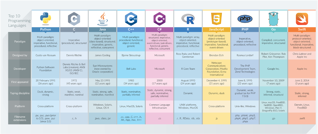
Figure 4.1: Top 10 programming languages and their applications according to DZone in 2017.

4.4 Programming in R

Some can be used for a range of purposes – others are more specific, e.g. HTML for website building. We will be using R and RStudio in this module as the main tool to complete specific tasks we need to do for our data analysis. There are a lot of different tools out there that you can use to achieve the same outcomes (as you have seen with QGIS, and no doubt had experience of using some statistics/spreadsheet software) but we choose to use this tool because it provides us with many advantages over these other tools.

What is important to understand is that R and RStudio are two different things: - R is our programming language, which we need to understand in terms of general principles, syntax and structure. - RStudio is our Integrated Development Environment (IDE), which we need to understand in terms of functionality and workflow. An IDE is simply a complicated way of saying “a place where I write and build scripts and execute my code”.

As you may know already, R is a free and open-source programming language, that originally was created to focus on statistical analysis. In conjunction with the development of R as a language, the same community created the RStudio IDE to execute this statistical programming. Together, R and RStudio have grown into an incredibly success partnership of analytical programming language and analysis software - and is widely used for academic research as well as in the commercial sector.

One of R’s great strength is that it is open-source, can be used on all major computer operating systems and is free for anyone to use. It, as a result, has a huge and active contributor community which constantly adds functionality to the language and software, making it an incredibly useful tool for many purposes and applications beyond statistical analysis.

Unlike traditional statistical analysis programmes you may have used such as Microsoft Excel or even SPSS, within the RStudio IDE, the user has to type commands to get it to execute tasks such as loading in a data set or performing a calculation. We primarily do this by building up a script, that provides a record of what you have done, whilst also enabling the straightforward repetition of tasks.

We can also use the R Console to execute simple instructions that do not need repeating - such as installing libraries or quickly viewing data (we will get to this in a second). In addition, R, its various graphic-oriented “packages” and RStudio are capable of making graphs, charts and maps through just a few lines of code (you might notice a Plots window to your right in your RStudio window) - which can then be easily modified and tweaked by making slight changes to the script if mistakes are spotted.

Unfortunately, command-line computing can also be off-putting at first. It is easy to make mistakes that are not always obvious to detect and thus debug. Nevertheless, there are good reasons to stick with R and RStudio. These include:

• It is broadly intuitive with a strong focus on publishable-quality graphics.
• It is ‘intelligent’ and offers in-built good practice – it tends to stick to statistical conventions and present data in sensible ways.
• It is free, cross-platform, customisable and extendable with a whole swathe of packages/libraries (‘add ons’) including those for discrete choice, multilevel and longitudinal regression, and mapping, spatial statistics, spatial regression, and geostatistics.
• It is well respected and used at the world’s largest technology companies (including Google, Microsoft and Facebook, and at hundreds of other companies).
• It offers a transferable skill that shows to potential employers experience both of statistics and of computing.

The intention of the practical elements of this week is to provide a thorough introduction to RStudio to get you started:

1. The basic programming principles behind R.
2. Loading in data from csv files, filtering and subsetting it into smaller chunks and joining them together.
3. Calculating a number of statistics for data exploration and checking.
4. Creating basic and more complex plots in order to visualise the distributions values within a dataset.

What you should remember is that R has a steep learning curve, but the benefits of using it are well worth the effort. The best way to really learn R is to take the basic code provided in tutorials and experiment with changing parameters - such as the colour of points in a graph - to really get ‘under the hood’ of the software.

4.4.1 The RStudio interface

You should all have access to some form of R - whether this is on your personal computer, Desktop@UCL Anywhere or through RStudio Server. If not, please go through the Geocomputation: An Introduction section. Go ahead and open RStudio and we will first take a quick tour of the various components of the RStudio environment interface and how and when to use them.

RStudio has various windows that you use for different purposes - and you can customise its layout dependent on your preference. When you first open RStudio, it should look a little something like this:

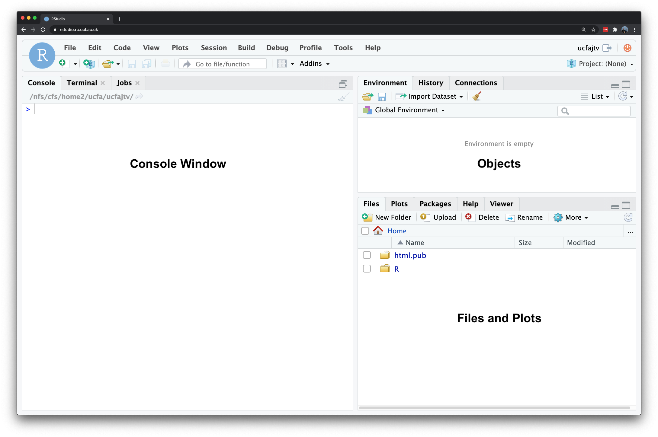
Figure 4.2: RStudio on RStudio Server.

The main windows (panel/pane) to keep focused on for now are:

• Console: where we write “one-off” code, such as installing libraries/packages, as well as running quick views or plots of our data.
• Files: where our files are stored on our computer system - can help with checking file paths as well as file names, and general file management.
• Environment: where our variables are recorded - we can find out a lot about our variables by looking at the environment window, including data structure, data type(s) and the fields and ‘attributes’ of our variables.
• Plots: the outputs of our graphs, charts and maps are shown here.
• Help: where you an search for help, e.g. by typing in a function to find out its parameters.

You may also have your Script Window open, which is where we build up and write code, to a) keep a record of our work, b) enable us to repeat and re-run code again, often with different parameters. We will not use this window until we get to the final practical instructions.

We will see how we use these windows as we progress through this tutorial and understand in more detail what we mean by words such as ‘attributes’ (do not get confused here with the Attribute Table for QGIS) and data structures.

4.5 RStudio console

We will first start off with using RStudio’s console to test out some of R’s in-built functionality by creating a few variables as well as a dummy data set that we will be able to analyse - and to get familiar with writing code.

Note
You might need to click on the console window to get it to expand - you can then drag it to take up a larger space in your RStudio window.

In your RStudio console, you should see a prompt sign - > to the left - this means we are ready to start writing code. Anything that appears as red in the command line means it is an error (or a warning) so you will likely need to correct your code. If you see a > on the left it means you can type in your next line, a + means that you have not finished the previous line of code. As will become clear, + signs often appear if you do not close brackets or you did not properly finish your command in a way that R expected.

In your console, let us go ahead and conduct some quick maths - at their most basic, all programming languages can be used like calculators.

4.5.1 Command Input

Type in 10 * 12 into the console.

# conduct some maths
10 * 12

## [1] 120

Once you press return, you should see the answer of 120 returned below.

4.5.2 Storing variables

Rather than use ‘raw’ or ‘standalone’ numbers and values, we primarily want to use variables that stores these values (or groups of them) under a memorable name for easy reference later. In R terminology this is called *creating an object and this object becomes stored as a variable**. The <- symbol is used to assign the value to the variable name you have given. Let us create two variables for experimenting with.

Type in ten <- 10 into the console and execute.

# store our ten variable
ten <- 10

You have just created your first variable. You will see nothing is returned in the console - but if you check your environment window, it has now appeared as a new variable that contains the associated value.

Type in twelve <- 12 into the console and execute.

# store our twelve variable
twelve <- 12

Once again, you will see nothing returned to the console but do check your environment window for your variable. We have now stored two numbers into our environment - and given them variable names for easy reference. R stores these objects as variables in your computer’s RAM so they can be processed quickly. Without saving your environment (we will come onto this below), these variables would be lost if you close R (or it crashes). Now we have our variables, we can go ahead and execute the same simple multiplication:

Type in ten * twelve into the console and execute.

# conduct some maths again using our variables
ten * twelve

## [1] 120

You should see the output in the console of 120.

Whilst this maths may look trivial, it is, in fact, extremely powerful as it shows how these variables can be treated in the same way as the values they contain.

Next, type in ten * twelve * 8 into the console and execute.

# conduct some more maths with variables and raw values
ten * twelve * 8

## [1] 960

You should get an answer of 960. As you can see, we can mix variables with raw values without any problems.

We can also store the output of variable calculations as a new variable. Type output <- ten * twelve * 8 into the console and execute.

# conduct some maths and store it as output
output <- ten * twelve * 8

As we are storing the output of our maths to a new variable, the answer is not returned to the screen.

4.5.3 Accessing and returning variables

We can ask our computer to return this output by simply typing it into the console. You should see we get the same value as the earlier equation.

# return the variable, output
output

## [1] 960

4.5.4 Variables of different data types

We can also store variables of different data types, not just numbers but text as well.

Type in str_variable <- "This is our first string variable" into the console and execute.

# store a variable
str_variable <- "This is our 1st string variable"

We have just stored our sentence made from a combination of characters, including letters and numbers. A variable that stores “words” (that may be sentences, or codes, or file names), is known as a string. A string is always denoted by the use of the quotation marks ("" or '').

Type in str_variable into the console and execute.

# return our str_variable
str_variable

## [1] "This is our 1st string variable"

You should see our entire sentence returned - and enclosed in quotation marks (""). Again, by simply entering our variable into the console, we have asked R to return our variable to us.

4.5.5 Calling functions on our variables

We can also call a function on our variable. This use of call is a very specific programming term and generally what you use to say “use” a function. What it simply means is that we will use a specific function to do something to our variable. For example, we can also ask R to print our variable, which will give us the same output as accessing it directly via the console.

Type in print(str_variable) into the console and execute.

# print str_variable to the screen
print(str_variable)

## [1] "This is our 1st string variable"

We have just used our first function: print(). This function actively finds the variable and then returns this to our screen. You can type ?print into the console to find out more about the print() function.

# gain access to the documentation for our print function
?print

This can be used with any function to get access to their documentation which is essential to know how to use the function correctly and understand its output. In many cases, a function will take more than one argument or parameter, so it is important to know what you need to provide the function with in order for it to work. For now, we are using functions that only need one argument.

4.5.6 Returning functions

When a function provides an output, such as this, it is known as returning. Not all functions will return an output to your screen - they will simply just do what you ask them to do, so often we require a print() statement or another type of returning function to check whether the function was successful or not. More on this later.

4.5.7 Examining our variables using functions

Within the base R language, there are various functions that have been written to help us examine and find out information about our variables. For example, we can use the typeof() function to check what data type our variable is.

Type in typeof(str_variable) into the console and execute.

# call the typeof() function on str_variable to return the data type of our variable
typeof(str_variable)

## [1] "character"

You should see the answer: character. As evident, our str_variable is a character data type. We can try testing this out on one of our earlier variables too.

Type in typeof(ten) into the console and execute.

# call the typeof() function on ten variable to return the data type of our
# variable
typeof(ten)

## [1] "double"

You should see the answer: double. As evident, our ten is a double data type.

For high-level objects that involve (more complicated) data structures, such as when we load a csv into R as a data frame, we are also able to check what class our object is, as follows:

Type in class(str_variable) into the console and execute.

# call the class() function on str_variable to return the object of our
# variable
class(str_variable)

## [1] "character"

In this case, you will get the same answer - character - because, in R, both its class and type are the same: a character. In other programming languages, you might have had string returned instead, but this effectively means the same thing.

Type in class(ten) into the console and execute.

# call the class() function on ten to return the object of our variable
class(ten)

## [1] "numeric"

In this case, you will get a different answer - numeric - because the class of this variable is numeric. This is because the class of numeric objects can contain either doubles (decimals) or integers (whole numbers). We can test this by asking whether our ten variable is an integer or not.

Type in is.integer(ten) into the console and execute.

# test our ten variable by asking if it is an integer
is.integer(ten)

## [1] FALSE

You should see we get the answer FALSE - as we know from our earlier typeof() function, our variable ten is stored as a double and therefore cannot be an integer.

Whilst knowing this might not seem important now, but when it comes to our data analysis, the difference of a decimal number versus a whole number can quite easily add bugs into our code. We can incorporate these tests into our code when we need to evaluate an output of a process and do some quality assurance testing of our data analysis.

We can also ask how long our variable is - in this case, we will find out how many different sets of characters (strings) are stored in our variable, str_variable.

Type in length(str_variable) into the console and execute.

# call the length() function on str_variable to return the length of our
# variable
length(str_variable)

## [1] 1

You should get the answer 1 - as we only have one set of characters. We can also ask how long each set of characters is within our variable, i.e. ask how long the string contained by our variable is.

Type in nchar(str_variable) into the console and execute.

# call the nchar() function on str_variable to return the length of each of our
# elements within our variable
nchar(str_variable)

## [1] 31

You should get an answer of 31.

4.5.8 Creating a two-element object

Let us go ahead and test these two functions a little further by creating a new variable to store two string sets within our object, i.e. our variable will hold two elements.

Type in two_str_variable <- c("This is our second variable", "It has two parts to it") into the console and execute.

# store a new variable with two items using the c() function
two_str_variable <- c("This is our second string variable", "It has two parts to it")

In this piece of code, we have created a new variable using the c() function in R, that stands for combine values into a vector or list. We have provided that function with two sets of strings, using a comma to separate our two strings - all contained within the function’s brackets (()). You should now see a new variable in your environment window which tells us it is a) chr: characters, b) contains two items, and c) lists those items.

Let us now try both our length() and nchar() on our new variable and see what the results are.

# call the length() function and nchar() function on our new variable
length(two_str_variable)

## [1] 2

nchar(two_str_variable)

## [1] 34 22

You should notice that the length() function now returned a 2 and the nchar() function returned two values of 34 and 22.

There is one final function that we often want to use with our variables when we are first exploring them, which is attributes() - as our variables are very simple, they currently do not have any attributes (you are welcome to type in the code and try) but it is a really useful function, which we will come across later on.

# call the attributes() function on our new variable
attributes(two_str_variable)

## NULL

Note
In addition to make notes about the functions you are coming across in the workshop, you should notice that with each line of code in the examples, an additional comment is used to explain what the code does. Comments are denoted using the hash symbol #. This comments out that particular line so that R ignores it when the code is run. These comments will help you in future when you return to scripts a week or so after writing the code - as well as help others understand what is going on when sharing your code. It is good practice to get into writing comments as you code and not leave it to do retrospectively. Whilst we are using the console, using comments is not necessary - but as we start to build up a script later on, you will find them essential to help understand your workflow in the future.

4.6 Simple analysis

The objects we created and played with above are very simple: we have stored either simple strings or numeric values - but the real power of R comes when we can begin to execute functions on more complex objects. R accepts four main types of data structures: vectors, matrices, data frames, and lists. So far, we have dabbled with a single item or a dual item vector - for the latter, we used the c() function to allow us to combine our two strings together within a single vector. We can use this same function to create and build more complex objects - which we can then use with some common statistical functions.

We are going to try this out by using a simple set of dummy data: we are going to use the total number of pages and publication dates of the various editions of Geographic Information Systems and Science for a brief analysis:

Book Edition	Year	Total Number of Pages
1st	2001	454
2nd	2005	517
3rd	2011	560
4th	2015	477

As we can see, we will ultimately want to store the data in a table as above (and we could easily copy this to a csv to load into R if we wanted). But we want to learn a little more about data structures in R, therefore, we are going to go ahead and build this table “manually”.

4.6.1 Housekeeping

First, let us clear up our workspace and remove our current variables. Type rm(ten, twelve, output, str_variable, two_str_variable) into the console and execute.

# clear our workspace
rm(ten, twelve, output, str_variable, two_str_variable)

You should now see we no longer have any variables in our window - we just used the rm() function to remove these variables from our environment and free up some RAM. Keeping a clear workspace is another recommendation of good practice moving forward. Of course, we do not want to get rid of any variables we might need to use later - but removing any variables we no longer need (such as test variables) will help you understand and manage your code and your working environment.

4.6.2 Atomic vectors

The first complex data object we will create is a vector. A vector is the most common and basic data structure in R and is pretty much the workhorse of R. Vectors are a collection of elements that are mostly of either character, logical integer or numeric data types. Technically, vectors can be one of two types:

• Atomic vectors (all elements are of the same data type)
• Lists (elements can be of different data types)

Although in practice the term “vector” most commonly refers to the atomic types and not to lists.

The variables we created above are actually vectors - however they are made of only one or two elements. We want to make complex vectors with more elements to them.

Let us create our first official “complex” vector, detailing the different total page numbers for GISS. Type giss_page_no <- c(454, 517, 560, 477) into the console and execute.

# store our total number of pages, in chronological order, as a variable
giss_page_no <- c(454, 517, 560, 477)

Type print(giss_page_no) into the console and execute to check the results.

# print our giss_page_no variable
print(giss_page_no)

## [1] 454 517 560 477

We can see we have our total number of pages collected together in a single vector. We could if we want, execute some statistical functions on our vector object.

# calculate the arithmetic mean on our variable
mean(giss_page_no)

## [1] 502

# calculate the median on our variable
median(giss_page_no)

## [1] 497

# calculate the range numbers of our variable
range(giss_page_no)

## [1] 454 560

We have now completed our first set of descriptive statistics in R. We now know that the average number of pages the GISS book has contain is 497 pages - this is of course truly thrilling stuff, but hopefully an easy example to get on-board with.

Let us see how we can build on our vector object by adding in a second vector object that details the relevant years of our book. Note that the total number of pages are entered in a specific order to correspond to these publishing dates (i.e. chronological), as outlined by the table above. As a result, we will need to enter the publication year in the same order.

Type giss_year <- c(2001, 2005, 2011, 2015) into the console and execute.

# store our publication years, in chronological order, as a variable
giss_year <- c(2001, 2005, 2011, 2015)

Type print(giss_year) into the console and execute.

# print our giss_year variable
print(giss_year)

## [1] 2001 2005 2011 2015

Of course, on their own, the two vectors do not mean much - but we can use the same c() function to combine the two together to create a matrix.

4.6.3 Matrices

In R, a matrix is simply an extension of the numeric or character vectors. They are not a separate type of object per se but simply a vector that has two dimensions. That is they contain both rows and columns. As with atomic vectors, the elements of a matrix must be of the same data type. As both our page numbers and our years are numeric, we can add them together to create a matrix using the matrix() function.

Type giss_year_nos <- matrix(c(giss_year, giss_page_no), ncol=2) into the console and execute.

# create a new matrix from our two vectors with two columns
giss_year_nos <- matrix(c(giss_year, giss_page_no), ncol = 2)
# note the inclusion of a new argument to our matrix: ncol=2 this stands for
# 'number of columns' and we want two

Type print(giss_year_nos) into the console and execute to check the result.

print(giss_year_nos)

##      [,1] [,2]
## [1,] 2001  454
## [2,] 2005  517
## [3,] 2011  560
## [4,] 2015  477

The thing about matrices - as you might see above - is that, for us, they do not have a huge amount of use. If we were to look at this matrix in isolation from what we know it represents, we would not really know what to do with it. As a result, we tend to primarily use Data Frames in R as they offer the opportunity to add field names to our columns to help with their interpretation.

Note
The function we just used above, ‘matrix()’, was the first function that we used that took more than one argument. In this case, the arguments the matrix needed to run were:

1. What data or data set should be stored in the matrix.
2. How many columns (ncol=) do we need to store our data in.

The function can actually accept several more arguments - but these were not of use for us in this scenario, so we did not include them. For almost any R package, the documentation will contain a list of the arguments that the function will takes, as well as in which format the functions expects these arguments and a set of usage examples.

Understanding how to find out what object and data type a variable is essential therefore to knowing whether it can be used within a function - and whether we will need to transform our variable into a different data structure to be used for that specific function. For any function, there will be mandatory arguments (i.e. it will not run without these) or optional arguments (i.e. it will run without these, as the default to this argument has been set usually to FALSE, 0 or NULL).

4.6.4 Dataframes

A data frame is an extremely important data type in R. It is pretty much the de-facto data structure for most tabular data and what we use for statistics. It also is the underlying structure to the table data (what we would call the attribute table in Q-GIS) that we associate with spatial data - more on this next week.

A data frame is a special type of list where every element of the list will have the same length (i.e. data frame is a “rectangular” list), Essentially, a data frame is constructed from columns (which represent a list) and rows (which represents a corresponding element on each list). Each column will have the same amount of entries - even if, for that row, for example, the entry is simply NULL.

Data frames can have additional attributes such as rownames(), which can be useful for annotating data, like subject_id or sample_id or even UID. In statistics, they are often not used - but in spatial analysis, these IDs can be very useful. Some additional information on data frames:

• They are usually created by read.csv() and read.table(), i.e. when importing the data into R.
• Assuming all columns in a data frame are of same type, a data frame can be converted to a matrix with data.matrix() (preferred) oras.matrix().
• You can also create a new data frame with data.frame() function, e.g. a matrix can be converted to a data frame.
• You can find out the number of rows and columns with nrow() and ncol(), respectively.
• Rownames are often automatically generated and look like 1, 2, …, n. Consistency in numbering of rownames may not be honoured when rows are reshuffled or subset.

Let us go ahead and create a new data frame from our matrix.

Type giss_df <- data.frame(giss_year_nos) into the console and execute.

# create a new dataframe from our matrix
giss_df <- data.frame(giss_year_nos)

We now have a data frame, we can use the View() function in R. Still in your console, type: View(giss_df)

# view our data frame
View(giss_df)

You should now see a table pop-up as a new tab on your script window. It is now starting to look like our original table - but we are not exactly going to be happy with X1 and X2 as our field names - they are not very informative.

4.6.5 Column names

We can rename our data frame column field names by using the names() function. Before we do this, have a read of what the names() function does. Still in your console, type: ?names

# get the help documentation for the names function
?names

As you can see, the function will get or set the names of an object, with renaming occurring by using the following syntax: names(x) <- value

The value itself needs to be a character vector of up to the same length as x, or NULL. We have two columns in our data frame, so we need to parse our names() function with a character vector with two elements. In the console, we shall enter two lines of code, one after another. First our character vector with our new names, new_names <- c("year", "page_nos"), and then the names() function containing this vector for renaming, names(giss_df) <- new_names:

# create a vector with our new column names
new_names <- c("year", "page_nos")
# rename our columns with our next names
names(giss_df) <- new_names

You can go and check your data frame again and see the new names using either View() function or by clicking on the tab at the top.

4.6.6 Adding columns

We are still missing one final column from our data frame - that is our edition of the textbook. As this is a character data type, we would not have been able to add this directly to our matrix - and instead have waited until we have our data frame to do so. This is because data frames can take different data types, unlike matrices - so let us go ahead and add the edition as a new column.

To do so, we follow a similar process of creating a vector with our editions listed in chronological order, but then add this to our data frame by storing this vector as a new column in our data frame. We use the $ sign with our code that gives us “access” to the data frame’s column - we then specify the column edition, which whilst it does not exist at the moment, will be created from our code that assigns our edition variable to this column.

Create a edition vector variable containing our textbook edition numbers - type and execute edition <- c("1st", "2nd", "3rd", "4th"). We then store this as a new column in our data frame under the column name edition by typing and executing giss_df$edition <- edition:

# create a vector with our editions
edition <- c("1st", "2nd", "3rd", "4th")

# add this vector as a new column to our data frame
giss_df$edition <- edition

Again, you can go and check your data frame and see the new column using either View() function or by clicking on the tab at the top or by typing giss_df in your console window.

# inspect
giss_df

##   year page_nos edition
## 1 2001      454     1st
## 2 2005      517     2nd
## 3 2011      560     3rd
## 4 2015      477     4th

Now we have our data frame, let us find out a little about it. We can first return the dimensions (the size) of our data frame by using the dim() function. In your console, type dim(giss_df) and execute.

# check our data frame dimensions
dim(giss_df)

## [1] 4 3

We can see we have four rows and three columns. We can also finally use our attributes() function to get the attributes of our data frame. In your console, type attributes(giss_df) and execute:

# check our data frame attributes
attributes(giss_df)

## $names
## [1] "year"     "page_nos" "edition" 
## 
## $row.names
## [1] 1 2 3 4
## 
## $class
## [1] "data.frame"

Before we leave the console and move to a script, we will enter one last line of code for now to install an additoinal R library, called tidyverse. Type in install.packages("tidyverse") into the console and execute.

# install the tidyverse library
install.packages("tidyverse")

Note
When working in R it is important to keep in mind that:

• R is case-sensitive so you need to make sure that you capitalise everything correctly if required.
• The spaces between the words do not matter but the positions of the commas and brackets do. Remember, if you find the prompt, >, is replaced with a + it is because the command is incomplete. If necessary, hit the escape (esc) key and try again.
• It is important to come up with good names for your objects. In the case of the majority of our variables, we used a underscore _ to separate the words. It is good practice to keep the object names as short as possible but they still need to be easy to read and clear what they are referring to. Be aware: you cannot start an object name with a number!
• If you press the up arrow in the command line you will be able to edit the previous lines of code you have inputted.

4.7 Crime analysis I

The last command you executed was the installation of a new R library: tidyverse. The tidyverse is a collection of packages that are specifically designed for data wrangling, management, cleaning, analysis and visualisation within RStudio. Whilst in many cases different packages work all slightly differently, all packages of the tidyverse share the underlying design philosophy, grammar, and data structures.

The tidyverse itself is treated and loaded as a single package, but this means if you load the tidyverse package within your script (through library(tidyverse)), you will directly have access to all the functions that are part of each of the packages that are within the overall tidyverse. This means you do not have to load each package separately. For more information on tidyverse, have a look at https://www.tidyverse.org/.

There are some specific functions in tidyverse suite of packages that will help us cleaning and preparing our data sets now and in the future - which is one of the main reasons of using this library. The most important and useful functions, from the tidyr and dplyr packages, are:

Package	Function	Use to
dplyr	select	select columns
dplyr	filter	select rows
dplyr	mutate	transform or recode variables
dplyr	summarise	summarise data
dplyr	group by	group data into subgropus for further processing
tidyr	pivot_longer	convert data from wide format to long format
tidyr	pivot_wider	convert long format data set to wide format

These functions all complete very fundamental tasks that we need to manipulate and wrangle our data.

Note
The tidyr and dplyr packages with the tidyverse are just two examples of additional libraries created by the wider R community. The code you just ran asked R to fetch and install the tidyverse into your copy of R - so this means we will be able to use these libraries in our practical below simply by using the library(tidyverse) code at the top of our script.

One thing we need to be aware of when it comes to using functions in these additional libraries, is that sometimes these functions are called the same thing as the base R package, or even, in some cases, another additional library. We therefore often need to specify which library we want to use this function from, and this can be done with a simple command (library::function) in our code.

Whilst we have gone ahead and installed the tidyverse, each time we start a new script, we will need to load the tidyverse.

4.7.1 Starting a project

In the previous section, R may have seemed fairly labour-intensive. We had to enter all our data manually and each line of code had to be written into the command line. Fortunately this is not routinely the case. In RStudio, we can use scripts to build up our code that we can run repeatedly - and save for future use. Before we start a new script, we first want to set up ourselves ready for the rest of our practicals by creating a new project.

To put it succinctly, projects in RStudio keep all the files associated with a project together — input data, R scripts, analytical results, figures. This means we can easily keep track of - and access - inputs and outputs from different weeks across our module, whilst still creating standalone scripts for each bit of processing analysis we do. It also makes dealing with directories and paths a whole lot easier - particularly if you have followed the folder structure that was advised at the start of the module.

Click on File -> New Project -> Existing Directory and browse to your GEOG0030 folder. Click on Create Project.

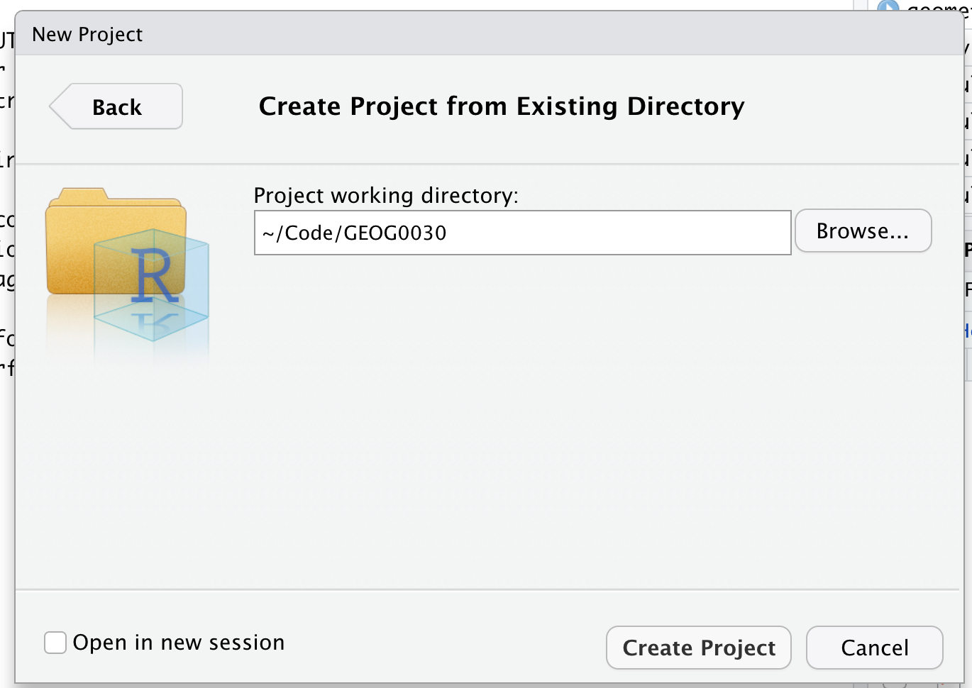
Figure 4.3: Create a new project in an existing directory.

You should now see your main window switch to this new project - and if you check your Files window, you should now see a new R Project called GEOG0030:

Figure 4.4: A new R project.

We are now “in” the GEOG0030 project - and any folders within the GEOG0030 project can be easily accessed by our code. Furthermore, any scripts we create will be saved in this project. Note, there is not a “script” folder per se, but rather your scripts will simply exist in this project.

Note
Please ensure that folder names and file names do not contain spaces or special characters such as * . " / \ [ ] : ; | = , < ? > & $ # ! ' { } ( ). Different operating systems and programming languages deal differently with spaces and special characters and as such including these in your folder names and file names can cause many problems and unexpected errors. As an alternative to using white space you can use an underscore _ if you like.

4.7.2 Setting up a script

For the majority of our analysis work, we will type our code within a script and not the console. Let us create our first script. Click on File -> New File -> R Script. This should give you a blank document that looks a bit like the command line. The difference is that anything you type here can be saved as a script and re-run at a later date.

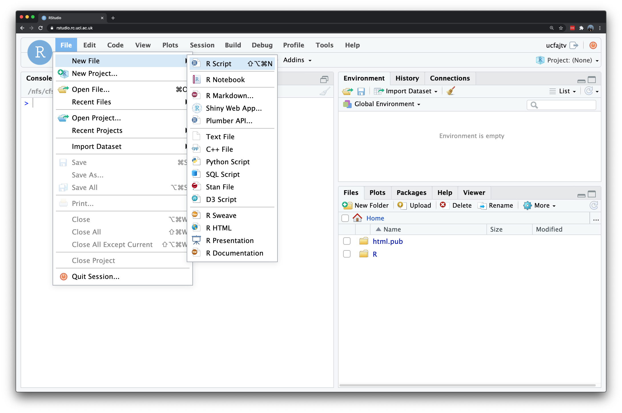
Figure 4.5: Creating a new script.

Save your script as: wk4-csv-processing.r. Through our name, we know now that our script was created in Week 4 of Geocomputation and the code it will contain is something to do with csv processing. This will help us a lot in the future when we come to find code that we need for other projects.

The first bit of code you will want to add to any script is to add a title. This title should give any reader a quick understanding of what your code achieves. When writing a script it is important to keep notes about what each step is doing. To do this, the hash (#) symbol is put before any code. This comments out that particular line so that R ignores it when the script is run.

Let us go ahead and give our script a title - and maybe some additional information:

# Combining Police Data csv's from 2020 into a single csv
# Followed by analysis of data on monthly basis
# Date: January 2022
# Author: Justin 

Now we have our title, the second bit of code we want to include in our script is to load our libraries (i.e. the installed packages we want to use in our script):

# libraries
library(tidyverse)

By loading simply the tidyverse, we have a pretty good estimate that we will be able to access all the functions that we are going to need today. However, often when developing a script, you will realise that you will need to add libraries as you go along in order to use a specific function etc. When you do this, always add your library to the top of your script - if you ever share your script, it helps the person you are sharing with recognise quickly if they need to install any additional packages prior to trying to run the script. It also means your libraries do not get lost in the multiple lines of code you are writing.

We are now ready to run these first two lines of code. Remember to save your script.

4.7.3 Running a script

There are two main ways to run a script in RStudio - all at once or by line/chunk by line/chunk. It can be advantageous to pursue with the second option as you first start out to build your script as it allows you to test your code iteratively.

To run line-by-line

By clicking:

• Select the line or chunk of code you want to run, then click on Code and choose Run selected lines.

By key commands:

• Select the line or chunk of code you want to run and then hold Ctl or Cmd and press Return.

To run the whole script

By clicking:

• Click on Run on the top-right of the scripting window and choose Run All.

By key commands:

• Hold Option plus Ctl or Cmd and R.

Stopping a script from running

If you are running a script that seems to be stuck (for whatever reason) or you notice some of your code is wrong, you will need to interrupt R. To do so, click on Session -> Interrupt R. If this does not work, you may end up needing to Terminate R but this may lose any unsaved progress.

4.7.4 Crime data

Where last week we provided you with a crime data set, this week you will download and prepare the data set yourself.

1. Start by navigating to data.police.uk. And click on Downloads.
2. Under the data range select January 2020 to December 2020.
3. Under the Custom download tab select Metropolitan Police Service and City of London Police. Leave all other settings and click on Generate file.

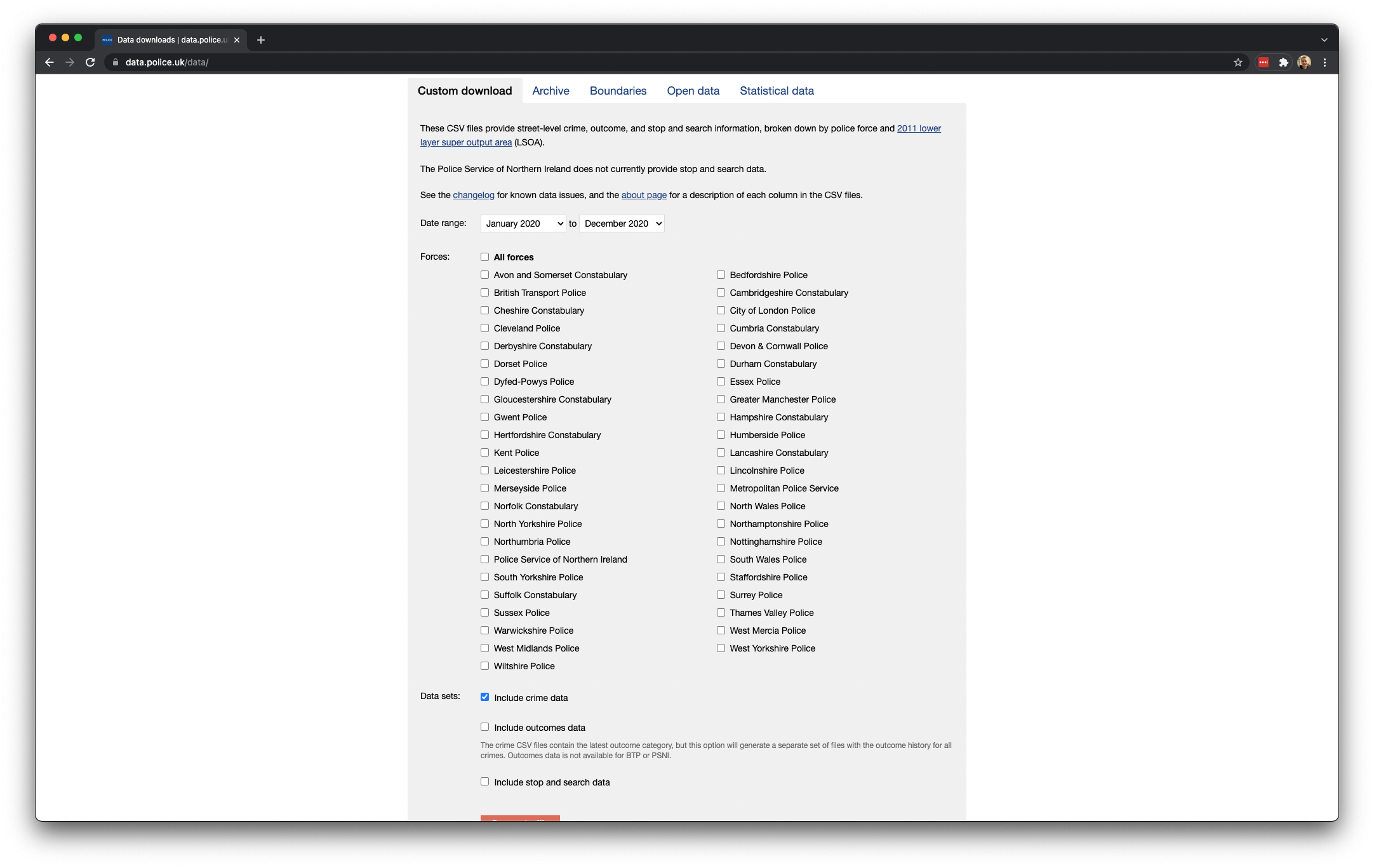
Figure 4.6: Downloading our crime data.

3. It may take a few minutes for the download to be generated, so be patient. Once the Download now button appears, you can download the 2020 crime data set.
4. Once downloaded, unzip the file. You will notice that the zip file contains 12 individual folders - one for each month in 2020. Each folder contains two files - one containing the data for the Metropolitan Police Service and one for the City of London Police.
5. Create a new folder named all_crime in your data/raw/crime directory and copy all 12 folders containing our data to this new folder.

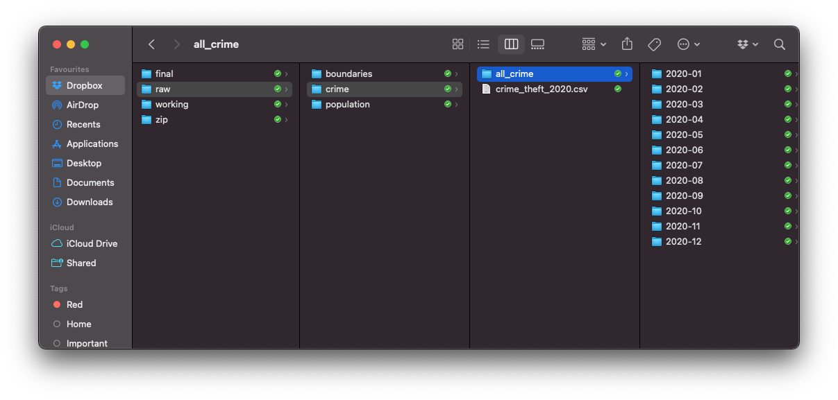
Figure 4.7: Your data folder should now look something like this.

4.7.4.1 Reading data into R

We are now ready to get started with using the crime data csv's currently sat in our all_crime folder. To do so, we need to first figure out how to import the csv and understand the data structure it will be in after importing. To read in a csv into R requires the use of a very simple function from the tidyverse library: read_csv().

We can look at the help documentation to understand what we need to provide the function (or rather the optional arguments), but as we just want to load single csv, we will go ahead and just use the function with a simple parameter.

# read in a single csv from our crime data
crime_csv <- read_csv("data/raw/crime/all_crime/2020-01/2020-01-metropolitan-street.csv")

Note
If using a Windows machine, you will need to submit your forward-slashes (/) with two backslashes (\\) whenever you are dealing with file paths!

We can explore the csv we have just loaded as our new crime_csv variable and understand the class, attributes and dimensions of our variable.

# check class and dimensions of our data frame
class(crime_csv)

## [1] "spec_tbl_df" "tbl_df"      "tbl"         "data.frame"

dim(crime_csv)

## [1] 90979    12

We have found out our variable is a data frame, containing 90979 rows and 12 columns. We however do not want just the single csv and instead what to combine all our csv's in our all_crime folder into a single data frame - so how do we do this?

This will be the most complicated section of code you will come across today, and we will use some functions that you have not seen before.

# read in all files and append all rows to a single data frame
all_crime_df <- list.files(path = "data/raw/crime/all_crime/", full.names = TRUE,
    recursive = TRUE) %>%
    lapply(read_csv) %>%
    bind_rows

This might take a little time to process (or might not), as we have a lot of data to get through. You should see a new data frame appear in your global environment called all_crime_df, for which we now have 1,187,847 observations!

Note
It is a little difficult to explain the code above without going into too much detail, but essential what the code does is:

1. List all the files found in the data path: data/raw/crime/all_crime/
2. Read each of these as a csv by “applying” the read_csv() function on all files.
3. Binding all rows of all individual data frames into a single data frame.

These three different actions are combined by using something called a pipe (%>%), which we will explain in more detail in later weeks.

4.7.4.2 Inspecting data in R

We can now have a look at our large dataframe in more detail.

# understand our all_crime_df cols, rows and print the first five rows
ncol(all_crime_df)

## [1] 12

nrow(all_crime_df)

## [1] 1187847

head(all_crime_df)

## # A tibble: 6 × 12
##   `Crime ID`    Month  `Reported by` `Falls within` Longitude Latitude Location 
##   <chr>         <chr>  <chr>         <chr>              <dbl>    <dbl> <chr>    
## 1 37c663d86a53… 2020-… City of Lond… City of Londo…   -0.106      51.5 On or ne…
## 2 5b89923fa5e0… 2020-… City of Lond… City of Londo…   -0.118      51.5 On or ne…
## 3 07172682a8b2… 2020-… City of Lond… City of Londo…   -0.112      51.5 On or ne…
## 4 14e02a6048af… 2020-… City of Lond… City of Londo…   -0.111      51.5 On or ne…
## 5 fb3350ce8e04… 2020-… City of Lond… City of Londo…   -0.113      51.5 On or ne…
## 6 <NA>          2020-… City of Lond… City of Londo…   -0.0976     51.5 On or ne…
## # … with 5 more variables: LSOA code <chr>, LSOA name <chr>, Crime type <chr>,
## #   Last outcome category <chr>, Context <lgl>

You should now see with have the same number of columns as our previous single csv, but with much more rows. You can also see that the head() function provides us with the first five rows of our data frame. You can conversely use tail() to provide the last five rows.

For now in our analysis, we only want to extract the theft crime in our data frame - so we will want to filter our data based on the Crime type column. However, as we can see, we have a space in our field name for Crime type and, in fact, many of the other fields. As we want to avoid having spaces in our field names when coding (or else our code will break!), we need to rename our fields. To do so, we will first get all of the names of our fields so we can copy and paste these over into our code:

# get the field names of our all_crime_df
names(all_crime_df)

##  [1] "Crime ID"              "Month"                 "Reported by"          
##  [4] "Falls within"          "Longitude"             "Latitude"             
##  [7] "Location"              "LSOA code"             "LSOA name"            
## [10] "Crime type"            "Last outcome category" "Context"

We can then rename the field names in our data set - just as we did with our GISS table earlier:

# create a new vector containing updated no space / no capital field names
no_space_names <- c("crime_id", "month", "reported_by", "falls_within", "longitude",
    "latitude", "location", "lsoa_code", "lsoa_name", "crime_type", "last_outcome_category",
    "context")

# rename our df field names using these new names
names(all_crime_df) <- no_space_names

We now have our dataframe ready for filtering - and to do so, we’ll use the filter() function from the dplyr library (which is library within our tidyverse). This function is really easy to use - but there is also a filter() function in the R base library - that does something different to the function in dplyr. As a result, we need to use a specific type of syntax - library::function - to tell R to look for and use the the filter function from the dplyr library rather than the default base library.

We then also need to populate our filter() function with the necessary parameters to extract only the “Theft from the person” crime type. This includes providing the function with our main data frame plus the filter query, as outliend below:

# filter all_crime_df to contain only theft, store as a new variable:
# all_theft_df
all_theft_df <- dplyr::filter(all_crime_df, crime_type == "Theft from the person")

You should now see the new variable appear in your environment with 31,578 observations. We now want to do some further housekeeping and create on final data frame that will allow us to analyse crime in London by month. To do so, we want to count how many thefts occur each month in London - and luckily for us dplyr has another function that will do this for us, known simply as count().

Go ahead and search the help to understand the count() function - you will also see that there is only one function called count() so far, i.e. the one in the dplyr library, so we do not need to use the additional syntax we used above.

Let us go ahead and count the number of thefts in London by month. The code for this is quite simple:

# count in the all_theft_df the number of crimes by month and store as a new
# dataframe
theft_month_df <- count(all_theft_df, month)

We have stored the output of our count() function to a new data frame: theft_month_df. Go ahead and look at the data frame to see the output - it is a very simple table containing simply the month and n, i.e. the number of thefts occurring per month. We can and should go ahead and rename this column to help with our interpretation of the data frame. We will use a quick approach to do this, that uses selection of the precise column to rename only the second column:

# rename the second column of our new data frame to crime_totals
names(theft_month_df)[2] <- "crime_totals"

This selection is made through the [2] element of code added after the names() function we have used earlier. We will look more at selection, slicing and indexing in next week’s practical.

4.8 Assignment

We now have our final data set ready for our simple analysis and answer some simple questions.

1. What is the average number of crimes per month in London in 2020?

2. What is the median number of crimes per month in London in 2020?

3. What are the minimum and maximum values of crime in London in 2020?

4. Besides descriptive statistics, it would be really useful to generate a simple chart. Use the documentation of the barplot() function to create the barplot below:

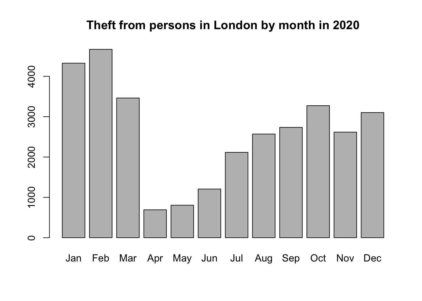
5. Do you notice anything interesting in the distribution of the theft from persons over time?
6. As this barplot is still a little basic, also try to figure out how to change the bar chart fill and borders to another colour from grey and black respectively.

Now, make sure to save your script, so we can return to it next week. You do not need to save your workspace - but can do so if you like. Saving the workspace will keep any variables generated during your current session saved and available in a future session.

4.9 Want more? [Optional]

The graphs and figures we have made so far are not really pretty. Although possible with the basic R installation, there are easier and better ways to make nice visualisations. For this we can turn to other R packages that have been developed. In fact, there are many hundreds of packages in R each designed for a specific purpose, some of which you can use to create plots in R. One of those packages is called ggplot2. The ggplot2 package is an implementation of the Grammar of Graphics (Wilkinson 2005) - a general scheme for data visualisation that breaks up graphs into semantic components such as scales and layers. ggplot2 can serve as a replacement for the base graphics in R and contains a number of default options that match good visualisation practice. You provide the data, tell ggplot2 how to map variables to aesthetics, what graphical primitives to use, and it takes care of the details. An excellent introduction to ggplot2 can be found in the online, freely available book R for Data Science; written by Hadley Wickham, core developer of ggplot2 and the tidyverse. Have a particularly close look at Chapter 3: Data visualisation: [Link].

4.10 Before you leave

We have managed to take a data set of over one million records and clean and filter it to provide a chart that actually shows the potential impact of the first COVID-19 lockdown on theft crime in London. Of course, there is a lot more research and exploratory data analysis we would need to complete before we could really substantiate our findings, but this first chart is certainly a step in the right direction. Next week, we will be doing a lot more with our data set - including a lot more data wrangling and of course spatial analysis, but hopefully this week has shown you want you can achieve with just a few lines of code. That concludes the tutorial for this week.