3 Point Pattern Analysis

This week, we will be focusing on point pattern analysis (PPA), which aims to detect clusters or patterns within a set of points. Through this analysis, we can measure density, dispersion, and homogeneity in point structures. Various methods exist for calculating and identifying these clusters, and today we will explore several of these techniques using our bike theft dataset from last week.

3.1 Lecture slides

The slides for this week’s lecture can be downloaded here: [Link]

3.2 Reading list

Essential readings

• Arribas-Bel, D., Garcia-López, M.-À., Viladecans-Marsal, E. 2021. Building(s and) cities: Delineating urban areas with a machine learning algorithm. Journal of Urban Economics 125: 103217. [Link]
• Cheshire, J. and Longley, P. 2012. Identifying spatial concentrations of surnames. International Journal of Geographical Information Science 26(2), pp.309-325. [Link]
• Longley, P. et al. 2015. Geographic Information Science & systems, Chapter 12: Geovisualization. [Link]

Suggested readings

• Van Dijk, J. and Longley, P. 2020. Interactive display of surnames distributions in historic and contemporary Great Britain. Journal of Maps 16, pp.58-76. [Link]
• Yin, P. 2020. Kernels and density estimation. The Geographic Information Science & Technology Body of Knowledge. [Link]

3.3 Start of session

Before working through the tutorial, we will spend a few minutes looking at:

• Identical coordinates among the bicycle theft points
• How spatstat stores point data differently to sf
• The difference between st_intersects() and st_intersection()

3.4 Bike theft in London II

This week, we will revisit bicycle theft in London, focusing specifically on identifying patterns and clusters of theft incidents. To do this, we will use the bicycle theft dataset that we prepared last week, along with the 2021 MSOA boundaries for London. If you no longer have a copy of these files on your computer, you can download them using the links provided below.

File	Type	Link
London Bicycle Theft 2025	GeoPackage	Download
London MSOA 2021 Spatial Boundaries	GeoPackage	Download

To get started, let us create our first script. File -> New File -> R Script. Save your script as w03-bike-theft.r.

We will start by loading the libraries that we will need:

R code

# load libraries
library(tidyverse)
library(sf)
library(tmap)
library(spatstat)
library(terra)
library(dbscan)

You may have to install some of these libraries if you have not used these before.

As always, we will start by loading our files into memory:

R code

# load msoa dataset
msoa21 <- st_read("data/spatial/London-MSOA-2021.gpkg")

Reading layer `London-MSOA-2021' from data source 
  `/Users/justinvandijk/Library/CloudStorage/Dropbox/UCL/Web/jtvandijk.github.io/GEOG0030/data/spatial/London-MSOA-2021.gpkg' 
  using driver `GPKG'
Simple feature collection with 1002 features and 8 fields
Geometry type: MULTIPOLYGON
Dimension:     XY
Bounding box:  xmin: 503574.2 ymin: 155850.8 xmax: 561956.7 ymax: 200933.6
Projected CRS: OSGB36 / British National Grid

# load bicycle theft dataset
theft_bike <- st_read("data/spatial/London-BicycleTheft-2025.gpkg")

Reading layer `London-BicycleTheft-2025' from data source 
  `/Users/justinvandijk/Library/CloudStorage/Dropbox/UCL/Web/jtvandijk.github.io/GEOG0030/data/spatial/London-BicycleTheft-2025.gpkg' 
  using driver `GPKG'
Simple feature collection with 14094 features and 10 fields
Geometry type: POINT
Dimension:     XY
Bounding box:  xmin: 212146 ymin: 53145.11 xmax: 580025 ymax: 398976
Projected CRS: OSGB36 / British National Grid

# inspect
head(msoa21)

Simple feature collection with 6 features and 8 fields
Geometry type: MULTIPOLYGON
Dimension:     XY
Bounding box:  xmin: 530966.7 ymin: 180512.6 xmax: 551943.8 ymax: 191139
Projected CRS: OSGB36 / British National Grid
   msoa21cd                 msoa21nm msoa21nmw  bng_e  bng_n      lat      long
1 E02000001       City of London 001           532384 181355 51.51562 -0.093490
2 E02000002 Barking and Dagenham 001           548267 189685 51.58652  0.138756
3 E02000003 Barking and Dagenham 002           548259 188520 51.57606  0.138149
4 E02000004 Barking and Dagenham 003           551004 186412 51.55639  0.176828
5 E02000005 Barking and Dagenham 004           548733 186824 51.56069  0.144267
6 E02000007 Barking and Dagenham 006           549698 186609 51.55851  0.158087
                                globalid                           geom
1 {71249043-B176-4306-BA6C-D1A993B1B741} MULTIPOLYGON (((532135.1 18...
2 {997A80A8-0EBE-461C-91EB-3E4122571A6E} MULTIPOLYGON (((548881.6 19...
3 {62DED9D9-F53A-454D-AF35-04404D9DBE9B} MULTIPOLYGON (((549102.4 18...
4 {511181CD-E71F-4C63-81EE-E8E76744A627} MULTIPOLYGON (((551550.1 18...
5 {B0C823EB-69E0-4AE7-9E1C-37715CF3FE87} MULTIPOLYGON (((549099.6 18...
6 {A33C6ADD-D70A-4737-ADE5-3460D7016CA1} MULTIPOLYGON (((549819.9 18...

# inspect
head(theft_bike)

Simple feature collection with 6 features and 10 fields
Geometry type: POINT
Dimension:     XY
Bounding box:  xmin: 531847 ymin: 181156 xmax: 533407 ymax: 181926.9
Projected CRS: OSGB36 / British National Grid
                                                          crime_id   month
1 f39615e054dd6ced4e7cac76acaaf0312429b67d1c944fddc6a165330c691de2 2025-01
2 342ec0e118067e0a88fc7c5fdf4b80520a3793ea625d0ab44ff5d87522d27025 2025-01
3 52983bbb3fa5f2c0faec4fa45ed12581bb5236aedad0553923d76b79290c8243 2025-01
4 b0de6b48cbd276a48ca2a41683c1fcf3cfbb6baf15289234ecf420b9e1e9112f 2025-01
5 0992e08fa4e37dc9ffea6905f6ec88b32a2f03ac5bac1a6d366a1b59bd9aea07 2025-01
6 93611647e6ea48308dcbb9f0ad59adc13661e66f301240d85c3806a660989ecf 2025-01
            reported_by          falls_within                 location
1 City of London Police City of London Police   On or near Silk Street
2 City of London Police City of London Police  On or near Milton Court
3 City of London Police City of London Police   On or near Houndsditch
4 City of London Police City of London Police On or near Pindar Street
5 City of London Police City of London Police    On or near New Change
6 City of London Police City of London Police    On or near Amen Court
  lsoa_code           lsoa_name    crime_type
1 E01000002 City of London 001B Bicycle theft
2 E01000002 City of London 001B Bicycle theft
3 E01000005 City of London 001E Bicycle theft
4 E01032739 City of London 001F Bicycle theft
5 E01032739 City of London 001F Bicycle theft
6 E01032739 City of London 001F Bicycle theft
                          last_outcome_category context                    geom
1 Investigation complete; no suspect identified      NA   POINT (532441 181911)
2 Investigation complete; no suspect identified      NA   POINT (532608 181849)
3                   Unable to prosecute suspect      NA   POINT (533407 181356)
4                   Unable to prosecute suspect      NA POINT (533182 181926.9)
5 Investigation complete; no suspect identified      NA   POINT (532182 181156)
6                   Unable to prosecute suspect      NA POINT (531847 181247.1)

You can further inspect both objects using the View() function.

3.4.1 Point aggregation

One key advantage of point data is that it is scale-free, allowing aggregation to any geographic level for analysis. Before diving into PPA, we will aggregate the bicycle thefts to the MSOA level to map their distribution by using a point-in-polygon approach.

R code

# point in polygon
msoa21 <- msoa21 |>
    mutate(theft_bike_n = lengths(st_intersects(msoa21, theft_bike, sparse = TRUE)))

To create a point-in-polygon count within sf, we use the st_intersects() function and keep its default sparse = TRUE output, which produces a list of intersecting points by index for each polygon (e.g. MSOA). We then apply the lengths() function to count the number of points intersecting each polygon, giving us the total number of bike thefts per MSOA.

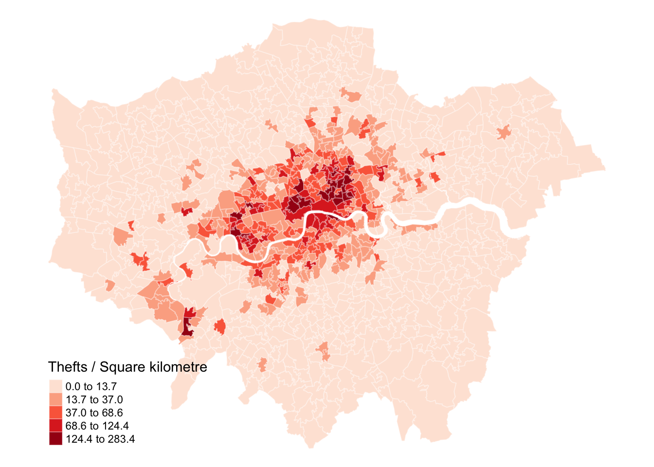
We can now calculate the area of each MSOA and, combined with the total number of bicycle thefts, determine the number of thefts per square kilometre. This involves calculating the size of each MSOA in square kilometres and then dividing the total number of thefts by this area to get a theft density measure.

R code

# msoa area size
msoa21 <- msoa21 |>
    mutate(km_sq = as.numeric(st_area(msoa21))/1e+06)

# theft density
msoa21 <- msoa21 |>
    mutate(thef_km_sq = theft_bike_n/km_sq)

Let’s put this onto a map:

R code

# shape
tm_shape(msoa21) +

  # map data
  tm_polygons(
    # map data
    fill = "thef_km_sq",
    fill.scale = tm_scale_intervals(
      n = 5, style = "jenks",
      values = c("#fee5d9", "#fcae91", "#fb6a4a", "#de2d26", "#a50f15")
    ),

    # legend
    fill.legend = tm_legend(
      title = "Share of population",
      na.text = "No population",
      frame = FALSE,
    ),

    # borders
    col = "#ffffff",
    col_alpha = 0.3
  ) +

  # layout
  tm_layout(
    # legend
    legend.title.size = 0.8,
    legend.text.size = 0.8,
    legend.position = c(0.8, 0.35),

    # canvas
    frame = FALSE
  )

Figure 1: Number of reported bicycle thefts by square kilometre.

3.4.2 Point pattern analysis

Figure 1 shows that the number of bicycle thefts is clearly concentrated in parts of Central London. While this map may provide helpful insights, its representation depends on the classification and aggregation of the underlying data. Alternatively, we can directly analyse the point events themselves. For this, we will use the spatstat library, the primary library for point pattern analysis in R. To use spatstat, we need to convert our data into a ppp object.

The ppp format is specific to spatstat but is also used in some other spatial analysis libraries. A ppp object represents a two-dimensional point dataset within a defined area, called the window of observation (owin in spatstat). We can either create a ppp object directly from a list of coordinates (with a specified window of observation) or convert it from another data type.

We can turn our theft_bike dataframe into a ppp object as follows:

R code

# london outline
outline <- msoa21 |>
    st_union()

# clip
theft_bike <- theft_bike |>
    st_intersection(outline)

Warning: attribute variables are assumed to be spatially constant throughout
all geometries

# sf to ppp
window = as.owin(msoa21)
theft_bike_ppp <- ppp(st_coordinates(theft_bike)[, 1], st_coordinates(theft_bike)[,
    2], window = window)

Warning: data contain duplicated points

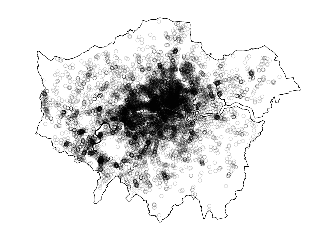
# inspect
par(mar = c(1, 1, 1, 1))
plot(theft_bike_ppp, main = "")

Figure 2: Bike theft in London represented as ppp object.

Some statistical procedures require point events to be unique. In our bicycle theft data, duplicates are likely due to the police snapping points to protect anonymity and privacy. This can pose an issue for spatial point pattern analysis, where each theft and its location must be distinct. We can check whether we have any duplicated points as follows:

R code

# check for duplicates
anyDuplicated(theft_bike_ppp)

[1] TRUE

# count number of duplicated points
sum(multiplicity(theft_bike_ppp) > 1)

[1] 8122

To address this, we have three options:

1. Remove duplicates if the number of duplicated points is small or the exact location is less important than the overall distribution.
2. Assign weights to points, where each has an attribute indicating the number of events at that location rather than being recorded as separate event.
3. Add jitter by slightly offsetting the points randomly, which can be useful if precise location is not crucial for the analysis.

Each approach has its own trade-offs, depending on the analysis. In our case, we will use the jitter approach to retain all bike theft events. Since the locations are already approximated, adding a small offset (~5 metre) will not impact the analysis.

R code

# add jitter
theft_bike_jitter <- rjitter(theft_bike_ppp, radius = 5, retry = TRUE, nsim = 1,
    drop = TRUE)

# check for duplicates
anyDuplicated(theft_bike_jitter)

[1] FALSE

# count number of duplicated points
sum(multiplicity(theft_bike_jitter) > 1)

[1] 0

This seemed to have worked, so we can move forward.

3.4.2.1 Kernel density estimation

Instead of visualising the distribution of bike thefts at a specific geographical level, we can use Kernel Density Estimation (KDE) to display the distribution of these incidents. KDE is a statistical method that creates a smooth, continuous distribution to represent the density of the underlying pattern between data points.

Kernel Density Estimation (KDE) generates a raster surface that shows the estimated density of event points across space. Each cell represents the local density, highlighting areas of high or low concentration. KDE uses overlapping moving windows (defined by a kernel) and a bandwidth parameter, which controls the size of the window, influencing the smoothness of the resulting density surface. The kernel function can assign equal or weighted values to points, producing a grid of density values based on these local calculations.

Let’s go ahead and create a simple KDE of bike theft with our bandwidth set to 500 metres:

R code

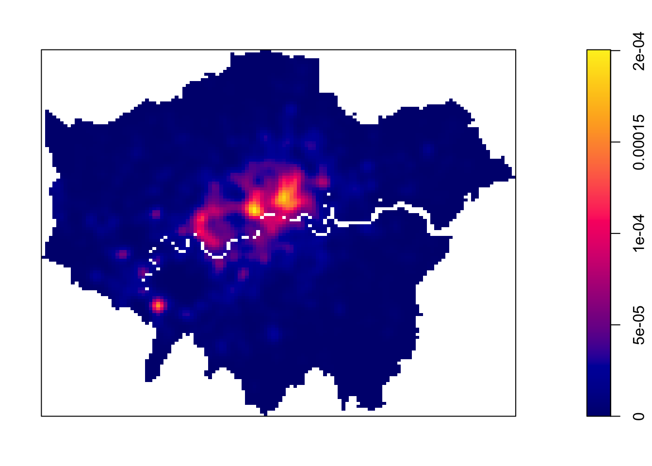
# kernel density estimation
par(mar = c(1, 1, 1, 1))
plot(density.ppp(theft_bike_jitter, sigma = 500), main = "")

Figure 3: Kernel density estimation - bandwidth 500m.

We can see from just our KDE that there are visible clusters present within our bike theft data, particularly in and around Central London. We can go ahead and increase the bandwidth to see how that affects the density estimate:

R code

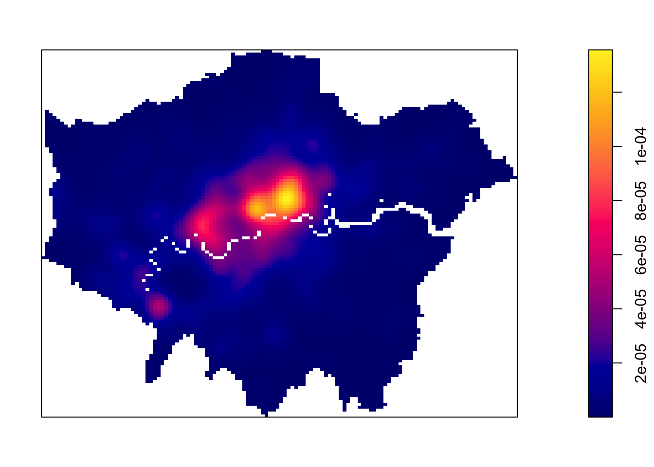
# kernel density estimation
par(mar = c(1, 1, 1, 1))
plot(density.ppp(theft_bike_jitter, sigma = 1000), main = "")

Figure 4: Kernel density estimation - bandwidth 1000m.

By increasing the bandwidth, our clusters appear larger and brighter than with the 500-metre bandwidth. A larger bandwidth considers more points, resulting in a smoother surface. However, this can lead to oversmoothing, where clusters become less defined, potentially overestimating areas of high bike theft. Smaller bandwidths offer more precision and sharper clusters but risk undersmoothing, which can cause irregularities.

While automated methods (e.g. maximum-likelihood estimation) can assist in selecting an optimal bandwidth, the choice is subjective and depends on the specific characteristics of your dataset.

Although bandwidth has a greater impact on density estimation than the kernel type, the choice of kernel can still influence the results by altering how points are weighted within the window. We will explore kernel types a little further when we discuss spatial models in a few weeks time.

Once we are satisfied with our KDE visualisation, we can create a proper map by converting the KDE output into raster format.

R code

# to raster
theft_bike_raster <- density.ppp(theft_bike_jitter, sigma = 1000) |>
    rast()

We now have a standalone raster that we can use with any function in the tmap library. However, one issue is that the resulting raster lacks a Coordinate Reference System (CRS), so we need to manually assign this information to the raster object:

R code

# set CRS
crs(theft_bike_raster) <- "EPSG:27700"

Now we can map the KDE values.

R code

# shape
tm_shape(theft_bike_raster) +

  # map data
  tm_raster(
    # map data
    col = "lyr.1",
    col.scale = tm_scale(
      values = "brewer.blues"
    ),

    # legend
    col.legend = tm_legend(
      title = "Density",
      frame = FALSE,
    )
  ) +

  # layout
  tm_layout(
    # legend
    legend.outside = FALSE,
    legend.position = c(0.8, 0.35),
    legend.text.size = 0.8,

    # canvas
    frame = FALSE
  )

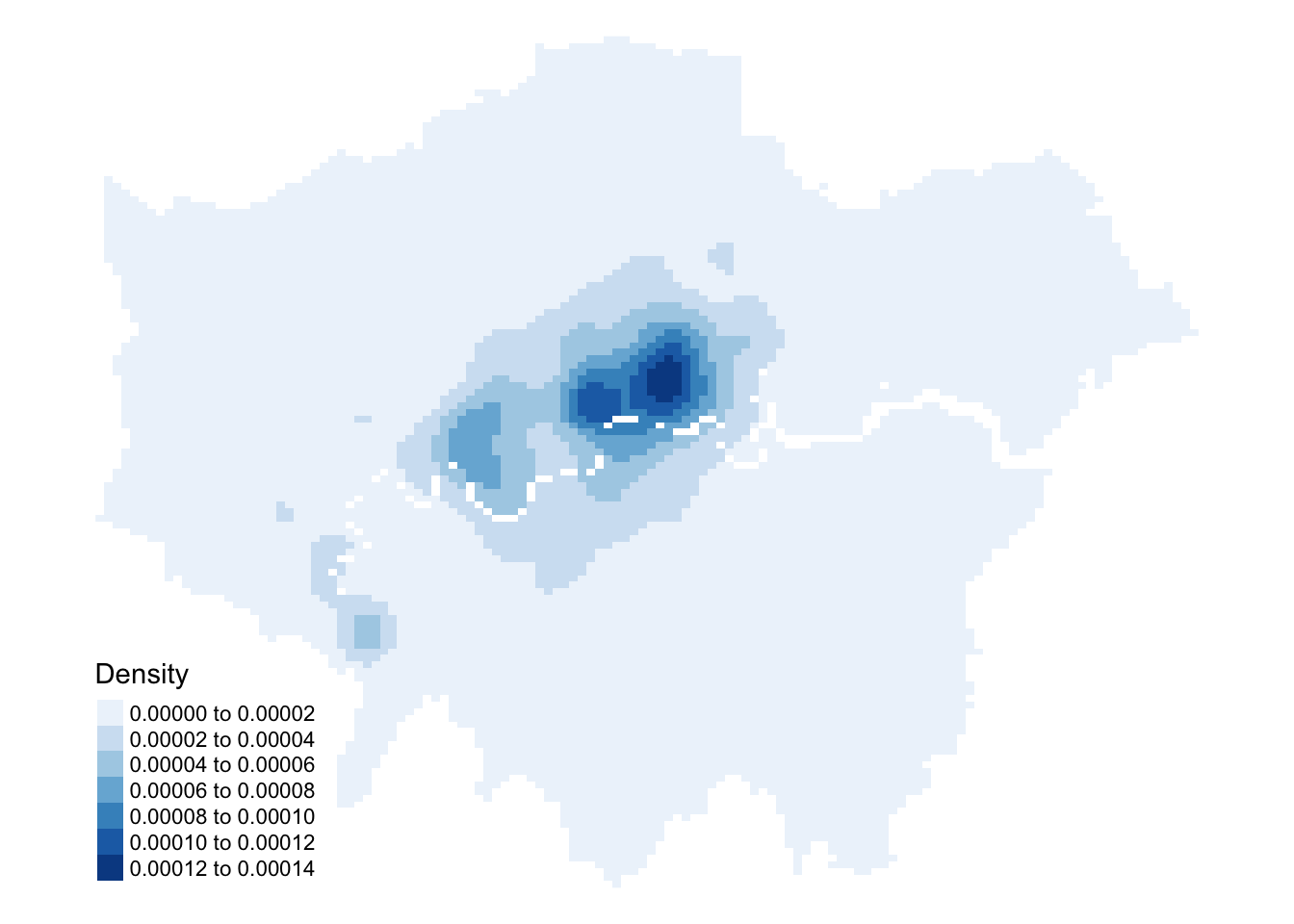
Figure 5: Kernel Density Estimate of bicycle thefts in London.

The values of the KDE output are stored in the raster grid as lyr.1.

3.4.2.2 DBSCAN

Kernel Density Estimation is a useful exploratory technique for identifying spatial clusters in point data, but it does not provide precise boundaries for these clusters. To more accurately delineate clusters, we can use an algorithm called DBSCAN (Density-Based Spatial Clustering of Applications with Noise), which takes both distance and density into account. DBSCAN is effective at discovering distinct clusters by grouping together points that are close to one another while marking points that do not belong to any cluster as noise.

DBSCAN requires two parameters:

Parameter	Description
epsilon	The maximum distance for points to be considered in the same cluster.
minPts	The minimum number of points for a cluster.

The algorithm groups nearby points based on these parameters and marks low-density points as outliers. DBSCAN is useful for uncovering patterns that are difficult to detect visually, but it works best when clusters have consistent densities.

Let us try this with an epsilon of 200 metres and minPts of 20 bicycle thefts:

R code

# dbscan
bike_theft_dbscan <- theft_bike |>
    st_coordinates() |>
    dbscan(eps = 200, minPts = 20)

The dbscan() function accepts a data matrix or dataframe of points, not a spatial dataframe. That is why, in the code above, we use the st_coordinates() function to extract the projected coordinates from the spatial dataframe.

The DBSCAN output includes three objects, one of which is a vector detailing the cluster each bike theft observation has been assigned to. To work with this output effectively, we need to add the cluster labels back to the original point dataset. Since DBSCAN does not alter the order of points, we can simply add the cluster output to the theft_bike spatial dataframe.

R code

# add cluster numbers
theft_bike <- theft_bike |>
    mutate(dbcluster = bike_theft_dbscan$cluster)

Now that each bike theft point in London is associated with a specific cluster, where appropriate, we can generate a polygon representing these clusters. To do this, we will use the st_convex_hull() function from the sf package, which creates a polygon that covers the minimum bounding area of a collection of points. We will apply this function to each cluster using a for loop, which allows us to repeat the process for each group of points and create a polygon representing the geometry of each cluster.

R code

# create an empty list to store the resulting convex hull geometries set the
# length of this list to the total number of clusters found
geometry_list <- vector(mode = "list", length = max(theft_bike$dbcluster))

# begin loop
for (cluster_index in seq(1, max(theft_bike$dbcluster))) {

    # filter to only return points for belonging to cluster n
    theft_bike_subset <- theft_bike |>
        filter(dbcluster == cluster_index)

    # union points, calculate convex hull
    cluster_polygon <- theft_bike_subset |>
        st_union() |>
        st_convex_hull()

    # add the geometry of the polygon to our list
    geometry_list[cluster_index] <- (cluster_polygon)

}

# combine the list
theft_bike_clusters <- st_sfc(geometry_list, crs = 27700)

While loops in R should generally be avoided for large datasets due to inefficiency, they remain a useful tool for automating repetitive tasks and reducing the risk of errors. For smaller datasets or tasks that cannot easily be vectorised, loops can still be effective and simplify the code.

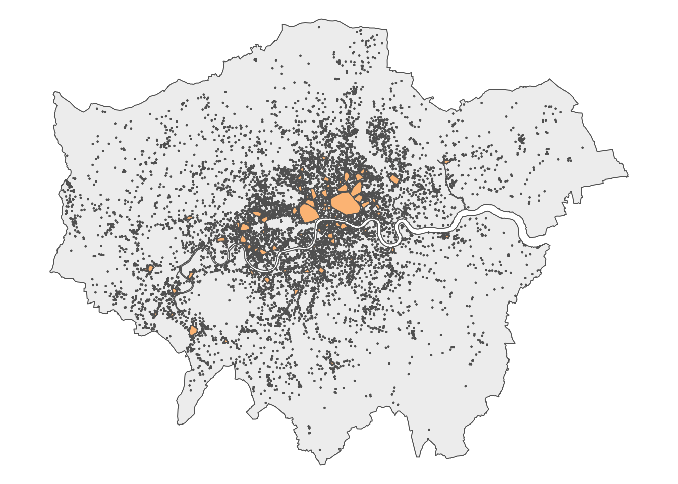
We now have a spatial dataframe that contains the bike theft clusters in London, as defined by the DBSCAN clustering algorithm. Let’s quickly map these clusters:

R code

# shape
tm_shape(outline) +

  # map data
  tm_polygons(
    fill = "#f0f0f0",
    col = NA
  ) +

  # shape
  tm_shape(theft_bike) +

  # map data
  tm_symbols(
    size = 0.10,
    fill = "#636363",
    col = "#636363",
  ) +

  # shape
  tm_shape(theft_bike_clusters) +

  # map data
  tm_polygons(
    col = "#fdc086",
    fill = "#fdc086",
    fill_alpha = 0.7
  ) +

  # layout
  tm_layout(
    frame = FALSE,
  )

Figure 6: DBSCAN-identified clusters of reported bicycle theft in London.

3.5 Assignment

Now that we know how to work with point location data, we can again apply a similar analysis to road crashes in London in 2025 that we used last week. This time we will use this dataset to assess whether road crashes cluster in specific areas. Try the following:

1. Choose a bandwidth for your Kernel Density Estimation (KDE) that you think best reveals clustering in all road crashes that occurred in London in 2025, and map the result.
2. Choose eps and minPts values for DBSCAN that you think reasonably define a cluster, and use the output to create a cluster map of serious and fatal road crashes in London.

If you no longer have a copy of the 2025 London STATS19 Road Collision dataset, you can download it using the link provided below.

File	Type	Link
London STATS19 Road Collisions 2025	csv	Download

3.6 Before you leave

With access to point event data, geographers aim to identify underlying patterns. This week, we explored several techniques that help us analyse and interpret such data. That is us done for this week. Reading list anyone?