1 Understanding data
1.1 Introduction
Welcome to your first week of Introduction to Quantitative Research Methods. This week we will focus on understanding data. We will also introduce you to some basic statistical terminology. Lastly, we will introduce you to the software tools that we will be using throughout this course: R and RStudio.
Note
Before you continue, make sure you have read through the details on the welcome page of this handbook and have watched the course introduction video.
This week is structured by 5 short videos, practical material that you need to work through in preparation for Thursday’s seminar, and a seminar task that you need to do in preparation for Thursday’s seminar.
Let’s get started.
Video: Introduction W01
[Lecture slides] [Watch on MS stream]1.1.1 Reading list
Please find the reading list for this week below. We strongly recommend that you read the core reading material before you continue with the rest of this week’s material.
Core reading
- Lane et al., 2003, Chapter 1: Introduction. In: Lane et al., 2003, Introduction to Statistics. Houston, Texas: Rice University. [Link]
Supplementary reading
- Diez et al., 2019, Chapter 1: Introduction to data. In: Diez et al., 2019, OpenIntro Statistics. Fourth Edition. Boston, Massachusetts: OpenIntro. [Link]
1.2 Data and statistics
Some of you may wonder why it is necessary to take a course on data and statistics in the first place? Well, there are several compelling reasons to have a (basic) knowledge of data and statistics:
- it will help you to understand and critically engage with academic articles;
- it will help you critically assess statistics used in the media, government reports, etc.;
- it will help you write a dissertation based on secondary analysis;
- it will help you write your own work convincingly.
Further to this, data skills are in high demand by employers both in the public and private sectors.
1.3 R for data analysis
Arguably the easiest way to start learning about data and statistics is by getting our hands dirty. So, before we will introduce you to some statistical terminology, we will have a look at one of the software tools with which we will be working this semester: R. R is a free software environment for statistical computing and graphics. It is extremely powerful and as such is now widely used for academic research as well as in the commercial sector. Ever wondered what tool is used to create those excellent coronavirus visualisations in the Financial Times?
R’s great strength is that it is open-source, can be used on all major computer operating systems and is free for anyone to use. Because of this, it is has rapidly become one of the statistical languages of choice for many academics. Moreover, it has a large and active user community with people constantly contributing new packages to carry out all manner of statistical and graphical analysis.
Unlike software programmes such as Microsoft Excel or SPSS, within a coding environment the user has to type commands to get it to execute tasks such as loading in a data set or performing a calculation. The biggest advantage of this approach is that you can build up a document, or script, that provides a record of what you have done, which in turn enables the straightforward repetition of tasks. Graphics can be easily modified and tweaked by making slight changes to the script or by scrolling through past commands and making quick edits. Unfortunately, command-line computing can also be off-putting at first. It is easy to make mistakes that are not always obvious to detect. Nevertheless, there are good reasons to stick with R. These include:
- It’s broadly intuitive with a strong focus on publishable-quality graphics.
- It’s ‘intelligent’ and offers in-built good practice – it tends to stick to statistical conventions and present data in sensible ways.
- It’s free, cross-platform, customisable and extendable with a whole swathe of libraries (‘add ons’) including those for discrete choice, multilevel and longitudinal regression, and mapping, spatial statistics, spatial regression, and geostatistics.
- It is well respected and used at the world’s largest technology companies (including Google, Microsoft and Facebook, and at hundreds of other companies).
- It offers a transferable skill that shows to potential employers experience both of statistics and of computing.
The intention of the practical elements of this week is to provide a thorough introduction to R to get you started:
- The basic programming principles behind R.
- Loading in data from
csvfiles and subsetting it into smaller chunks. - Calculating a number of statistics for data exploration and checking.
- Creating basic and more complex plots in order to visualise the distributions values within a data set.
R has a steep learning curve, but the benefits of using it are well worth the effort. Take your time and think through every piece of code you type in. The best way to learn R is to take the basic code provided in tutorials and experiment with changing parameters - such as the colour of points in a graph - to really get ‘under the hood’ of the software. Take lots of notes as you go along and if you are getting really frustrated take a break!
POLS0008 forum
If you encounter a problem during the course, e.g. something is unclear or you are stuck with your R code, you can post your question on the POLS0008 Forum. If you do not have questions yourself, do check the forum regularly as you may be able to help fellow students. Of course, the answers are moderated by the module tutors and the brilliant teaching support staff.
Some tips about how to get the best out of the forum:
- Be efficient, but also be polite. It just makes it a nicer read for all of us if you start with a greeting and end on a thanks, etc.!
- Be clear in the subject about what you are asking about. Topics named “Final Task” and “Same Problem”, for example, will get confusing very fast. We want the forum to be a lasting record of the module and there maybe something on there you want to refer back to so having descriptive subjects helps. For example “Boxplot does not have any whiskers” or “Unable to load in csv file” is better.
- Concisely outline the problem and also the steps you have taken to solve it. Explain what you are trying to do and why. This is really helpful for us to troubleshoot. As we will be using a programming language during the computer tutorials, the mistake you made might have happened a few lines of code before the one that is showing the error. We won’t know this without some extra context.
- Include the R code - a screenshot is fine but show the whole screen: there can be some useful clues in the console and objects list that we won’t see if you are showing only one line of code.
- If we solve a problem acknowledge this with a reply! How will we know otherwise?
- If you think you know the answer to someone’s question help them out!
- If you are having a similar issue post to the forum - including what you have done to try and fix it.
1.4 R console
You can download and install R on your laptop but for the purposes of this course we would like you to use the version hosted on the UCL servers so that everyone participating in the course has access to the same version of the software. Open a web browser and navigate to: https://rstudio.data-science.rc.ucl.ac.uk/ Log in with your usual UCL username and password. You should see the RStudio interface appear. If it is the first time you log on to RStudio server you may only see the RStudio interface appear once you have clicked on the start a new session button.s
Note
RStudio server will only work with an active VPN connection that links your personal computer into UCL’s network. Students in mainland may want to use UCL China Connect. Students that use a Mac computer that is running on the latest version of MacOS (MacOS Big Sur), are advised to use Desktop@UCL as the Cisco AnyConnect VPN application may not work. If you are completely unable to access the server (e.g. your browser displays a This site can’t be reached message), it means that your VPN connection is not working correctly. Please ensure that your VPN is working correctly or use Desktop@UCL Anywhere instead.
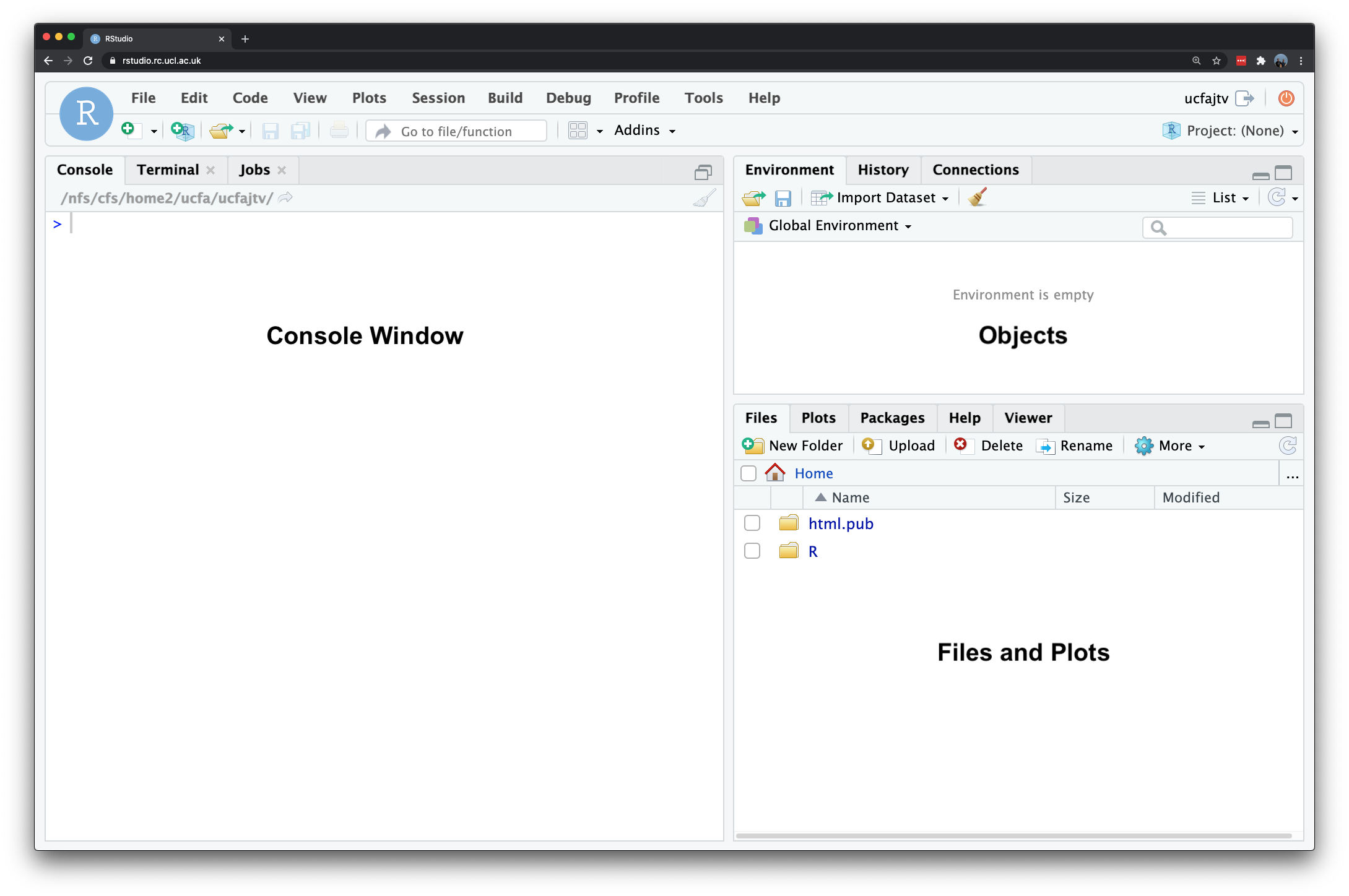
Figure 1.1: The RStudio interface.
If you managed to log onto RStudio server: brilliant, we are ready to go. At its absolute simplest R is a calculator, so let’s try adding some numbers by typing in the console window and hitting enter to execute the code:
4 + 10## [1] 14You will notices that in the command line window, it will give you an answer directly (i.e. 14). These outputs of the command line window are shown as ## throughout this handbook and you do not need to type anything into the command line that follows ## (because it simply shows the result of a command!).
Note
Anything that appears as red in the command line means it is an error (or a warning) so you will likely need to correct your code. If you see a > on the left it means you can type in your next line, a + means that you haven’t finished the previous line of code. As will become clear, + signs often appear if you don’t close brackets or you did not properly finish your command in a way that R expected.
Rather than using numbers and values, it is often easier to assign numbers (or groups of them) a memorable name for easy reference later. In R terminology this is called creating an object and this is really important. Let’s try this:
a <- 4
b <- 10
The <- symbol is used to assign the value to the name, in the above we assigned the integer 4 to an object with the name a. Similarly, we assigned the integer 10 to an object with the name b To see what each object contains you can just type print(name of your object), so in our case:
print(a)## [1] 4print(b)## [1] 10This may look trivial, but in fact it is extremely powerful as objects can be treated in the same way as the numbers they contain. For instance:
a*b## [1] 40Or even used to create new objects:
ab <- a*b
print(ab)
## [1] 40You can generate a list of objects that are currently active using the ls() command. R stores objects in your computer’s RAM so they can be processed quickly. Without saving (we will come onto this below) these objects will be lost if you close R (or it crashes).
ls()## [1] "a" "ab" "b"You may wish to delete an object. This can be done using rm() with the name of the object in the brackets. For example:
rm(ab)To confirm that your command has worked, just run the ls() command again:
ls()## [1] "a" "b"Note
Remember that if you have any questions with your R code and you are stuck that you can post a question on the POLS0008 Forum!
Let’s now take a short break from RStudio and have a look at some theory: the video below will introduce you to some essential statistical terminology.
Video: Statistical terminology
[Lecture slides] [Watch on MS stream]Now we now a little more about different types of variables and levels of measurement, we can go back to RStudio. Until now our objects have been extremely simple integers (i.e. whole numbers), but the real power of R comes when we can begin to execute functions on objects.
Let’s have a closer look at functions by firstly building a more complex object through the c() function. The c in the c() function means concatenate and essentially groups things together. Let’s create an object that contains the birth years of the six main characters in the popular American television sitcom Friends.
friends_dob <- c(1969,1967,1970,1968,1968,1967)Let’s check the results.
print(friends_dob)## [1] 1969 1967 1970 1968 1968 1967Now, we can execute some statistical functions on this object such as calculating the mean() value, the median() value, and the range() of the data.
mean(friends_dob)## [1] 1968.167median(friends_dob)## [1] 1968range(friends_dob)## [1] 1967 1970Note
In next week’s material we will dive a little deeper into these statistical functions, for now, however, we only want you to know how to execute a function. If at this stage you are not entirely sure on what what exactly is a range, median, or mean that is perfectly fine and you should not worry about it just yet.
All functions need a series of arguments to be passed to them in order to work. These arguments are typed within the brackets and typically comprise the name of the object (in the examples above its the friends_dob) that contains the data followed by some parameters. The exact parameters required are listed in the functions help files. To find the help file for the function type ? followed by the function name, for example:
?meanAll helpfiles will have a usage heading detailing the parameters required. In the case of the mean you can see it simply says mean(x, ...). In function helpfiles x will always refer to the object the function requires and, in the case of the mean, the ... refers to some optional arguments that we don’t need to worry about.
Note
When you are new to R the help files can seem pretty impenetrable (because they often are!). Up until relatively recently these were all people had to go on, but in recent years R has really taken off and so there are plenty of places to find help and tips. Google is the best tool to use. When people are having problems they tend to post examples of their code online and then the R community will correct it. One of the best ways to solve a problem is to paste their correct code into your R command line window and then gradually change it for your data and purposes.
The structure of the friends_dob object - essentially a group of numbers (integers!) - is known as a vector object in R. To build more complex objects that, for example, resemble a spreadsheet with multiple columns of data, it is possible to create a class of objects known as a data frame. This is probably the most commonly used class of object in R. We can create one here by combining two vectors.
friends_characters <- c('Monica','Ross','Rachel','Joey','Chandler','Phoebe')
friends <- data.frame(friends_characters, friends_dob)
If you type print(friends) you will see our newly created data frame that consists of the first vector object (date of birth) and the second vector objects (names of characters).
print(friends)## friends_characters friends_dob
## 1 Monica 1969
## 2 Ross 1967
## 3 Rachel 1970
## 4 Joey 1968
## 5 Chandler 1968
## 6 Phoebe 1967Tips
- R is case sensitive so you need to make sure that you capitalise everything correctly if required.
- The spaces between the words don’t matter but the positions of the commas and brackets do. Remember, if you find the prompt,
>, is replaced with a+it is because the command is incomplete. If necessary, hit the escape (esc) key and try again. - It is important to come up with good names for your objects. In the case of the
friends_dobobject we used a underscore_to separate the words. It is good practice to keep the object names as short as posssible so we could have gone forFriendsDoborf_dob. Be aware: you cannot start an object name with a number! - If you press the up arrow in the command line you will be able to edit the previous lines of code you inputted.
Recap
In this section you have:
- Entered your first commands into the R command line interface.
- Created objects in R.
- Created a vector of values (the
friends_dobobject). - Executed some simple R functions.
- Created a data frame (called
friends).
1.5 R script
In the previous section, R may have seemed fairly labour-intensive. We had to enter all our data manually and each line of code had to be written into the command line. Fortunately this isn’t routinely the case. In RStudio look to the top left corner and you will see a plus symbol, click on it and select R Script.
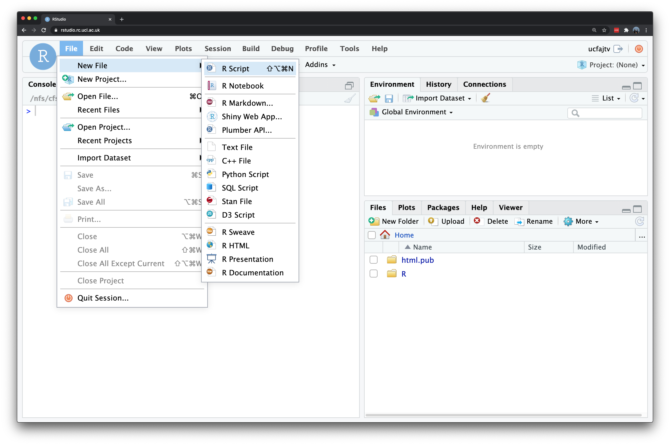
Figure 1.2: Opening a new script in RStudio.
This should give you a blank document that looks a bit like the command line. The difference is that anything you type here can be saved as a script and re-run at a later date.
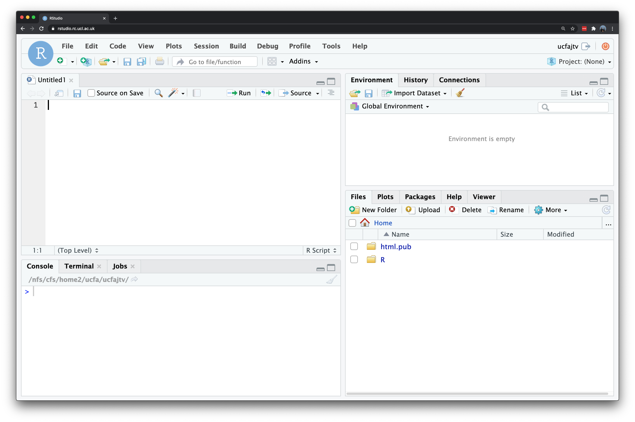
Figure 1.3: The RStudio interface with a new script.
When writing a script it is important to keep notes about what each step is doing. To do this the hash (#) symbol is put before any code. This comments out that particular line so that R ignores it when the script is run. Type the following into the scripting window:
# first attempt at creating a script
Some.Data <- data.frame(0:10,20:30)

# inspect the result
print(Some.Data)
Questions
- Without running these lines of code, what do you expect to happen? Do you understand what these simple line of codes do?
In the scripting window if you highlight all the code you have written and press the Run button on the top on the scripting window you will see that the code is sent to the command line and the text on the line after the # is ignored. From now on you should type your code in the scripting window and then use the Run button to execute it. If you have an error then edit the line in the script and hit run again.
Try it:
# first attempt at creating a script
Some.Data <- data.frame(0:10,20:30)
print(Some.Data)
## X0.10 X20.30
## 1 0 20
## 2 1 21
## 3 2 22
## 4 3 23
## 5 4 24
## 6 5 25
## 7 6 26
## 8 7 27
## 9 8 28
## 10 9 29
## 11 10 30The My.Data object is a data frame in need of some sensible column headings. You can add these by typing:
# add column names
names(Some.Data)<- c('x','y')

# print the object to check names were added successfully
print(Some.Data)
## x y
## 1 0 20
## 2 1 21
## 3 2 22
## 4 3 23
## 5 4 24
## 6 5 25
## 7 6 26
## 8 7 27
## 9 8 28
## 10 9 29
## 11 10 30Until now we have generated the data used in the examples above. One of R’s great strengths is its ability to load in data from almost any file format. Comma Separated Value (csv) files are our preferred choice. These can be thought of as stripped down Excel spreadsheets. They are an extremely simple format so they are easily machine readable and can therefore be easily read in and written out of R. As some of you may have never heard of a csv file before, in the video below we will look at csv files in a little more detail.
Video: csv files
[Lecture slides] [Watch on MS stream]
Working Directory
Since we are now reading and writing files it is good practice to tell R what your working directory is. Your working directory is the folder on the computer where you wish to store the data files you are working with. You can create a folder called POLS0008, for example. If you are using RStudio, on the lower right of the screen is a window with a Files tab. If you click on this tab you can then navigate to the folder you wish to use. You can then click on the More button and then Set as Working Directory. You should then see some code similar to the below appear in the command line. It is also possible to type the code in manually.
# set the working directory path to the folder you wish to use
# you may need to create the folder first if it doesn't exist
setwd('~/POLS0008')
# note the single / (\\ will also work)
Note
Please ensure that folder names and file names do not contain spaces or special characters such as * . " / \ [ ] : ; | = , < ? > & $ # ! ' { } ( ). Different operating systems and programming languages deal differently with spaces and special characters and as such including these in your folder names and file names can cause many problems and unexpected errors. As an alternative to using white space you can use an underscore _ if you like.
Once the working directory is setup it is then possible to load in a csv file. We are going to load a data set that has been saved in the working directory we just set that shows London’s historic population for each of its Boroughs. You can download the csv file below. The csv file is also available on Moodle in the data sets for practicals folder.
File download
| File | Type | Link |
|---|---|---|
| Borough Population London | csv |
Download |
Once downloaded to your own computer, this file will then need to be uploaded into RStudio. To do this click on the Upload button in the files area of the screen. Select the csv file you just downloaded and press OK. We can then type the following to locate and load in the file we need.
# load csv file from working directory
London.Pop <- read.csv('census-historic-population-borough.csv')
To view the object type:s
print(London.Pop)## Area.Code Area.Name Persons.1801 Persons.1811 Persons.1821
## 1 00AA City of London 129000 121000 125000
## Persons.1831 Persons.1841 Persons.1851 Persons.1861 Persons.1871
## 1 123000 124000 128000 112000 75000
## Persons.1881 Persons.1891 Persons.1901 Persons.1911 Persons.1921
## 1 51000 38000 27000 20000 14000
## Persons.1931 Persons.1939 Persons.1951 Persons.1961 Persons.1971
## 1 11000 9000 5000 4767 4000
## Persons.1981 Persons.1991 Persons.2001 Persons.2011 Borough.Type
## 1 5864 4230 7181 7375 1
## [ reached 'max' / getOption("max.print") -- omitted 32 rows ]Or if you only want to see the top 10 or bottom 10 rows you can use the head() and tail() functions. These are particularly useful if you have large data sets!
# view first 10 rows
head(London.Pop)
## Area.Code Area.Name Persons.1801 Persons.1811 Persons.1821
## 1 00AA City of London 129000 121000 125000
## Persons.1831 Persons.1841 Persons.1851 Persons.1861 Persons.1871
## 1 123000 124000 128000 112000 75000
## Persons.1881 Persons.1891 Persons.1901 Persons.1911 Persons.1921
## 1 51000 38000 27000 20000 14000
## Persons.1931 Persons.1939 Persons.1951 Persons.1961 Persons.1971
## 1 11000 9000 5000 4767 4000
## Persons.1981 Persons.1991 Persons.2001 Persons.2011 Borough.Type
## 1 5864 4230 7181 7375 1
## [ reached 'max' / getOption("max.print") -- omitted 5 rows ]# view bottom 10 rows
tail(London.Pop)## Area.Code Area.Name Persons.1801 Persons.1811 Persons.1821 Persons.1831
## 28 00BE Southwark 116000 139000 175000 207000
## Persons.1841 Persons.1851 Persons.1861 Persons.1871 Persons.1881
## 28 243000 292000 346000 407000 514000
## Persons.1891 Persons.1901 Persons.1911 Persons.1921 Persons.1931
## 28 572000 596000 579000 571000 535000
## Persons.1939 Persons.1951 Persons.1961 Persons.1971 Persons.1981
## 28 456000 338000 313413 262000 211858
## Persons.1991 Persons.2001 Persons.2011 Borough.Type
## 28 198916 244867 288283 1
## [ reached 'max' / getOption("max.print") -- omitted 5 rows ]Note
Depending on the type of object the exact number of lines displayed through head() and tail() may differ. If you want to have precise control over the output and specify how many rows will be printed, you can do this by passing an integer as second argument to either of these functions. For instance, head(London.Pop, n=10) or tail(London.Pop, n=10).
To learn a bit more about the file you have loaded, R has a number of useful functions. We can use these to find out how many columns (variables) and rows (cases) the data frame (data set) contains.
# get the number of columns
ncol(London.Pop)
## [1] 25# get the number of rows
nrow(London.Pop)## [1] 33# list the column headings
names(London.Pop)## [1] "Area.Code" "Area.Name" "Persons.1801" "Persons.1811"
## [5] "Persons.1821" "Persons.1831" "Persons.1841" "Persons.1851"
## [9] "Persons.1861" "Persons.1871" "Persons.1881" "Persons.1891"
## [13] "Persons.1901" "Persons.1911" "Persons.1921" "Persons.1931"
## [17] "Persons.1939" "Persons.1951" "Persons.1961" "Persons.1971"
## [21] "Persons.1981" "Persons.1991" "Persons.2001" "Persons.2011"
## [25] "Borough.Type"Given the number of columns in the pop data frame, subsetting by selecting on the columns of interest would make it easier to handle. In R there are two was of doing this. The first uses the $ symbol to select columns by name and then create a new data frame object.
# select the columns containing the Borough names and the 2011 population
London.Pop.2011 <- data.frame(London.Pop$Area.Name, London.Pop$Persons.2011)

# inspect the results
head(London.Pop.2011)
## London.Pop.Area.Name London.Pop.Persons.2011
## 1 City of London 7375
## 2 Barking and Dagenham 185911
## 3 Barnet 356386
## 4 Bexley 231997
## 5 Brent 311215
## 6 Bromley 309392A second approach to selecting particular data is to use [Row, Column] and ‘slice’ the data frame. For instance:
# select the 1st row of the 2nd column
London.Pop[1,2]
## [1] City of London
## 33 Levels: Barking and Dagenham Barnet Bexley Brent Bromley ... Westminster# select the first 5 rows of the 1st column
London.Pop[1:5,1]## [1] 00AA 00AB 00AC 00AD 00AE
## 33 Levels: 00AA 00AB 00AC 00AD 00AE 00AF 00AG 00AH 00AJ 00AK 00AL ... 00BK# select the first 5 rows of columns 8 to 11
London.Pop[1:5,8:11]## Persons.1851 Persons.1861 Persons.1871 Persons.1881
## 1 128000 112000 75000 51000
## 2 8000 8000 10000 13000
## 3 15000 20000 29000 41000
## 4 12000 15000 22000 29000
## 5 5000 6000 19000 31000# assign the previous selection to a new object
London.Subset <- London.Pop[1:5,8:11]In the code snippet, note how the colon : is used to specify a range of values. We used the same technique to create the Some.Data object above. The ability to select particular columns means we can see how the population of London’s Boroughs have changed over the past century by subtracting two columns from one another.
# within the brackets you can add additional columns to the data frame
# as long as their separated by commas
Pop.Change <- data.frame(London.Pop$Area.Name, London.Pop$Persons.2011 - London.Pop$Persons.1911)
If you type head(PopChange) you will see that the population change column (created to the right of the comma above) has a very long name. This can be changed using the names() command in the same way as we did this for our Some.Data object.
names(Pop.Change) <- c('Borough', 'Change_1911_2011')Since we have done some new analysis and created additional information it would be good to save the PopChange object to our working directory as a new csv file. This is done using the code below. Within the brackets we put the name of the R object we wish to save on the left of the comma and the file name on the right of the comma (this needs to be in inverted commas). Remember to put .csv after since this is the file format we are saving in.
write.csv(Pop.Change, 'Population_Change_1911_2011.csv')Recap
In this section you have learnt how to:
- Create an R script.
- Load a
csvinto R, perform some analysis, and write out a newcsvfile to your working directory. - Subset R data frames by name and also column and/or row number.
1.6 Seminar
Please find the seminar task and seminar questions for this week’s seminar below.
Note
Please make sure that you have executed the seminar task and have answered the seminar questions before the seminar!
Seminar task
Create a csv file that contains the following columns:
- The names of the London Boroughs.
- Population change between 1811 and 1911.
- Population change between 1911 and 1961.
- Population change between 1961 and 2011.
Seminar questions
Answer the following questions:
- Which Boroughs had the fastest growth between 1911 and 1961, and which had the slowest?
- You may have noticed that there is an additional column in the pop data frame called
Borough-Type. This indicates if a Borough is in inner (1) or outer (2) London. Is this variable ordinal or nominal?
Seminar link
Seminars for all groups take place on Thursday morning. You can find the Zoom link to your seminar group on Moodle in the Seminar links folder.
1.7 Before you leave
Save your R script by pressing the Save button in the script window. That is it for this week!