2 Statistical Inference and Causality
2.1 Introduction
Statistical inference is the process of using data analysis to deduce properties of an underlying distribution of probability. In other words: statistical inference is the procedure through which we try to make inferences about a population based on characteristics of this population that have been captured in a sample. This includes uncovering the association between variables as well as establishing causal relationships. However, correlation does not imply causation and identifying causal relationships from observational data is not trivial.
“Correlation does not imply causation” (Any statistician).
This week we will dive a little deeper into statistical inference and how to establish causal relationships by taking a small dive into the field of study of econometrics.
This week’s lecture video is provided by an absolute expert in the field of econometrics: Dr Idahosa from the University of Johannesburg. This week is further structured by reading material, a tutorial in R with a ‘hands-on’ application of the techniques covered in the lecture video, and a seminar on Tuesday.
Let’s get to it!
Video: Introduction W01
[Lecture slides] [Watch on MS stream]2.1.1 Reading list
Please find the reading list for this week below.
Core reading
- Bzdok, D., Altman, and M. Krzywinski. 2018. Statistics versus machine learning. Nature Methods 15: 233-234. [Link]
- Idahosa, L. O., Marwa, N., and J. Akotey. 2017. Energy (electricity) consumption in South African hotels: A panel data analysis. Energy and Buildings 156: 207-217. [Link]
- Stock, J. and M. Watson. 2019. Chapter 1: Economic Questions and Data. In: Stock, J. and M. Watson. Introduction to Econometrics, pp.43-54. Harlow: Pearson Education Ltd. [Link]
- Stock, J. and M. Watson. 2019. Chapter 10: Regression with Panel Data. In: Stock, J. and M. Watson. Introduction to Econometrics, pp.362-382. Harlow: Pearson Education Ltd. [Link]
Supplementary reading
- Idahosa, L. O. and J. T. van Dijk. 2016. South Africa: Freedom for whom? Inequality, unemployment and the elderly. Development 58(1): 96-102. [Link]
2.1.2 Technical Help session
Every Thursday between 13h00-14h00 you can join the Technical Help session on Microsoft Teams. The session will be hosted by Alfie. He will be there for the whole hour to answer any question you have live in the meeting or any questions you have formulated beforehand. If you cannot make the meeting, feel free to post the issue you are having in the Technical Help channel on the GEOG0125 Team so that Alfie can help to find a solution.
2.2 Statistical inference
Where during the remainder of this module we will predominantly focus on different machine learning methods and techniques and the data scientist’s toolbox, this week we will focus on statistical inference. Although there is considerable overlap between machine learning and statistics, sometimes even involving the same methods, the major difference between machine learning and statistics is their purpose. Where machine learning models are designed to make accurate predictions, statistical models are designed for inference about the relationships between variables.
“Statistics draws population inferences from a sample, and machine learning finds generalizable predictive patterns” (Bzdok et al. 2018).
One way to analyse the relationships between variables is by a linear regression. Linear regression models offer a very interpretable way to model the association between variables. A linear regression model is used to find the line that minimises the mean squared error across all data to establish the relationship between a response variable one or more explanatory (independent) variables. The case of one explanatory variable is called a simple linear regression; if more explanatory variables are used it is called multiple regression. The purpose of a regression model is to predict a target variable \(Y\) according to some other variable \(X\) or variables \(X_{1}\), \(X_{2}\), etc.
2.3 Causality
2.3.1 What is causality?
Regression cares about correlation: what happens to \(Y\) when \(X=x\). However, correlation does not imply causation. A great example can be found in a research project reporting on the relationships between chocolate consumption and the probability of winning a Nobel price. The results suggest that countries in which the population consumes on average a large amount of chocolate per annum, spawn more Nobel laureates per capita than countries in which the population on average consume less chocolate. There is a clear correlation in the data, but there should not exist an actual causal relationship between these two variables (Well, some research suggests it still remains unclear whether the correlation is spurious or whether it is an indication for hidden variables …)
The golden standard to establish a causal relationship is to set-up and execute a randomised control trial. Think of the many large-scale randomised control trials that are currently taking place to test the safety and effectiveness of various candidate coronavirus vaccines. However, it is not always possible to set up a randomised control trial. Sometimes this has to do with the nature of the relationship being investigated (e.g. establishing the effects of policy changes), but there could also be financial and ethical constraints. As an alternative, one could try to identify causal relationship from observational data. This is known as causal inference and most research in econometrics is concerned with retrieving valid estimates using different regression methods.
Note
The distinction between causal and non-causal relationships is crucial and heavily depends on your research questions. If you are trying to classify Google Street view images and predict whether the photo contains an office building or a residential building, you want to create a model that predicts this as good as possible. However, you do not care about what caused the building in the photo to be an office building or a residential building. That being said: almost any question is causal and where statistics is used in almost any field of inquiry, few pay proper attention to understanding causality.
By now you may wonder, sure, but what then is causality? We can say that \(X\) causes \(Y\) if we were to change the value of \(X\) without changing anything else then as a result \(Y\) would also change. A simple example: if you switch on the light switch, your light bulb will go on. The action of flipping the light switch causes your light to go on. This being said: it does not mean that \(X\) is necessarily the only thing that causes \(Y\) (e.g. the light bulb is burnt out or the light was already on) and perhaps a better way of phrasing it is to say that there is a causal relationship between variables if \(X\) changes the probability of \(Y\) happening or changing.
2.3.2 The problem with causality
The problem with establishing a causal relationship is that in many cases you cannot ‘switch on’ or ‘switch off’ a characteristic. Let’s go through this by thinking whether some \(X\) causes \(Y\). Our \(X\) is coded as 0 or 1, for instance, 0 if a person has not received a coronavirus vaccination and 1 if a person has received a coronavirus vaccination. \(Y\) is some numeric value. So how do we check if \(X\) causes \(Y\)? What we would need to do for everyone in our sample is to check what happens to \(Y\) when we make \(X=0\) and what happens to \(Y\) when we make \(X=1\). Obviously, this is a problem! You cannot both have \(X=0\) and \(X=1\): you either got inoculated against the coronavirus or you did not. This means that if \(X=1\) you can measure what the value of \(Y\) is, but you do not know what the value of \(Y\) would have been if \(X=0\). The solution you may come up with is to compare \(Y\) between individuals who have \(X=0\) and \(X=1\). However, there is another problem: there could be all kinds of reasons on why \(Y\) differs between individuals that are not necessarily related to \(X\).
Note
This section heavily borrows material and explanations from Nick Huntington-Klein’s excellent ECON 305: Economics, Causality, and Analytics module, do have a look if you want to learn more about this topic.
This brings us to econometrics and causal inference: the main goal of causal inference is to make the best possible estimation of what \(Y\) would have been if \(X\) would have been different, the so-called counterfactual. As we cannot always use an experiment in which we can randomly assign \(X\) so that we know that on average people with \(X=1\) and the same as people with \(X=2\), we have to come up with a model to figure out what the counterfactual would do.
In the following, we will explore two ways of doing this through so-called fixed effects models and random effects models in the situation in which we have data points for each observation across time (i.e. longitudinal data or panel data).
2.3.3 Fixed effects models
Fixed effects are variables that are constant across individuals; these variables, like age, sex, or ethnicity, typically do not change over time or change over time at a constant rate. As such, they have fixed effects on a dependent variable \(Y\). As such, using a fixed effects model you can explore the relationship between variables within an entity (which could be persons, companies, countries, etc.). Each entity has its own individual characteristics that may or may not influence the dependent variable. When using a fixed effects model, we assume that something within the entity may impact or bias the dependent variables and we need to control for this. A fixed effects model does this by removing the characteristics that do not change over time so that we can assess the net effect of the independent variables on the dependent variable.
Let’s try to to apply a fixed effects model in R. For this we will use a data set containing some panel data. The data set contains fictional data, for different countries and years, for an undefined variable \(Y\) that we want to explain with some other variables.
File download
| File | Type | Link |
|---|---|---|
| Example Panel Data | csv |
Download |
# load libraries
library(tidyverse)
library(plm)
library(car)
library(gplots)
library(tseries)
library(lmtest)

# read data
country_data <- read_csv('raw/w02/paneldata.csv')

# inspect
head(country_data)
## # A tibble: 6 x 6
## country year y x1 x2 x3
## <chr> <dbl> <dbl> <dbl> <dbl> <dbl>
## 1 A 1990 1342787840 0.278 -1.11 0.283
## 2 A 1991 -1899660544 0.321 -0.949 0.493
## 3 A 1992 -11234363 0.363 -0.789 0.703
## 4 A 1993 2645775360 0.246 -0.886 -0.0944
## 5 A 1994 3008334848 0.425 -0.730 0.946
## 6 A 1995 3229574144 0.477 -0.723 1.03Upon inspecting the dataframe you can see that the data contains 8 different fictional countries. For each country we have several years of data: three independent variables names \(X_{1}\), \(X_{2}\), and \(X_{3}\) and a dependent variable \(y\). As this is a panel dataset we have to declare it as such using the plm.data() function from the plm package. The plm package is a library dedicated to panel data analysis.
# create a panel data object
country_panel <- pdata.frame(country_data, index=c('country','year'))

# inspect
country_panel
## country year y x1 x2 x3
## A-1990 A 1990 1342787840 0.2779037 -1.1079559 0.28255358
## A-1991 A 1991 -1899660544 0.3206847 -0.9487200 0.49253848
## A-1992 A 1992 -11234363 0.3634657 -0.7894840 0.70252335
## A-1993 A 1993 2645775360 0.2461440 -0.8855330 -0.09439092
## A-1994 A 1994 3008334848 0.4246230 -0.7297683 0.94613063
## [ reached 'max' / getOption("max.print") -- omitted 65 rows ]Although the data looks the same, you can see that the row index has been updated to reflect the country and year variables. Let’s inspect the data using a boxplot as well as a conditioning plot. A coplot is a method for visualising interactions in your data set: it shows you how some variables are conditional on some other set of variables. So, for our panel data set, we can look at the variation of \(Y\) over time by country. The bars at top indicate the countries position from left to right starting on the bottom row.
# create a quick box plot
scatterplot(y ~ year, data=country_panel)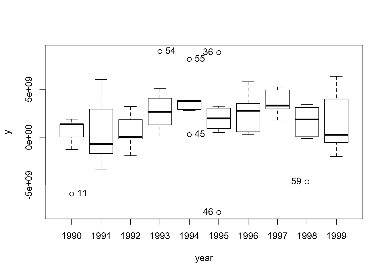
## [1] "11" "54" "45" "55" "46" "36" "59"# create a quick conditioning plot
coplot(y ~ year|country, data=country_panel, type='b')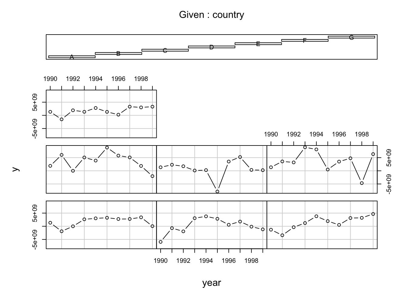
The graphs show that there \(Y\) is variable both over time and between countries. Let’s also have a look at the heterogeneity of our data by plotting the means, and the 95% confidence interval around the means, of \(Y\) across time and across countries.
# means across years
plotmeans(y ~ year, data=country_panel)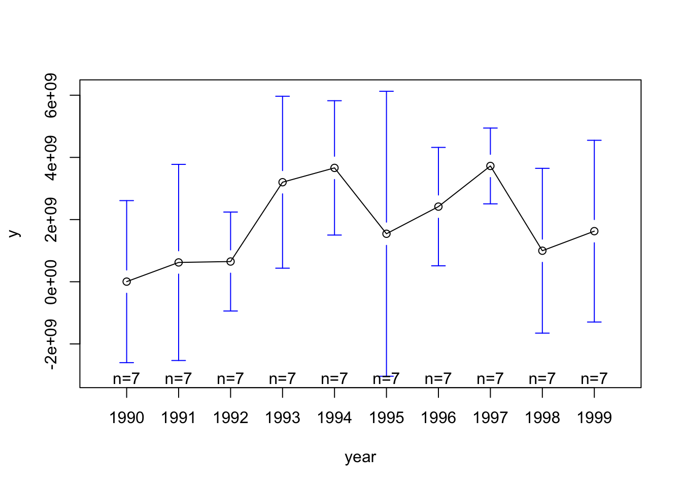
# means across countries
plotmeans(y ~ country, data=country_panel)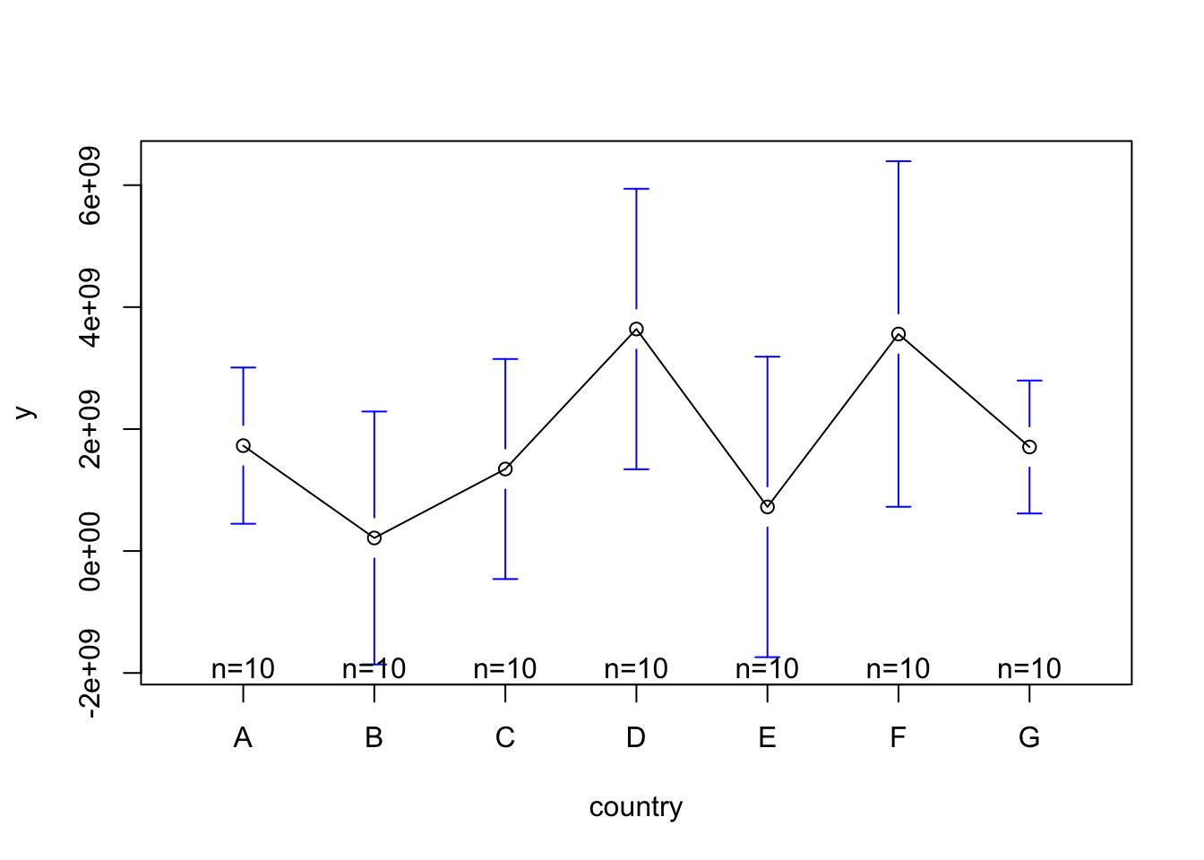
There is clearly some heterogeneity across the countries and across years. However, the basic Ordinary Least Squares (OLS) regression model does not consider this heterogeneity:
# run an OLS
ols <- lm(y ~ x1, data=country_panel)

# summary
summary(ols)
##
## Call:
## lm(formula = y ~ x1, data = country_panel)
##
## Residuals:
## Min 1Q Median 3Q Max
## -9.546e+09 -1.578e+09 1.554e+08 1.422e+09 7.183e+09
##
## Coefficients:
## Estimate Std. Error t value Pr(>|t|)
## (Intercept) 1.524e+09 6.211e+08 2.454 0.0167 *
## x1 4.950e+08 7.789e+08 0.636 0.5272
## ---
## Signif. codes: 0 '***' 0.001 '**' 0.01 '*' 0.05 '.' 0.1 ' ' 1
##
## Residual standard error: 3.028e+09 on 68 degrees of freedom
## Multiple R-squared: 0.005905, Adjusted R-squared: -0.008714
## F-statistic: 0.4039 on 1 and 68 DF, p-value: 0.5272The results show that there is no significant statistical relationship between \(X_{1}\) and the dependent variable \(Y\) as the model tries to explain all variability in the data at once. You can clearly see this in the plot below:
# plot the results
scatterplot(country_panel$y ~ country_panel$x1, boxplots=FALSE, smooth=FALSE, pch=19, col='black')

# add the OLS regression line
abline(lm(y ~ x1, data=country_panel),lwd=3, col='red')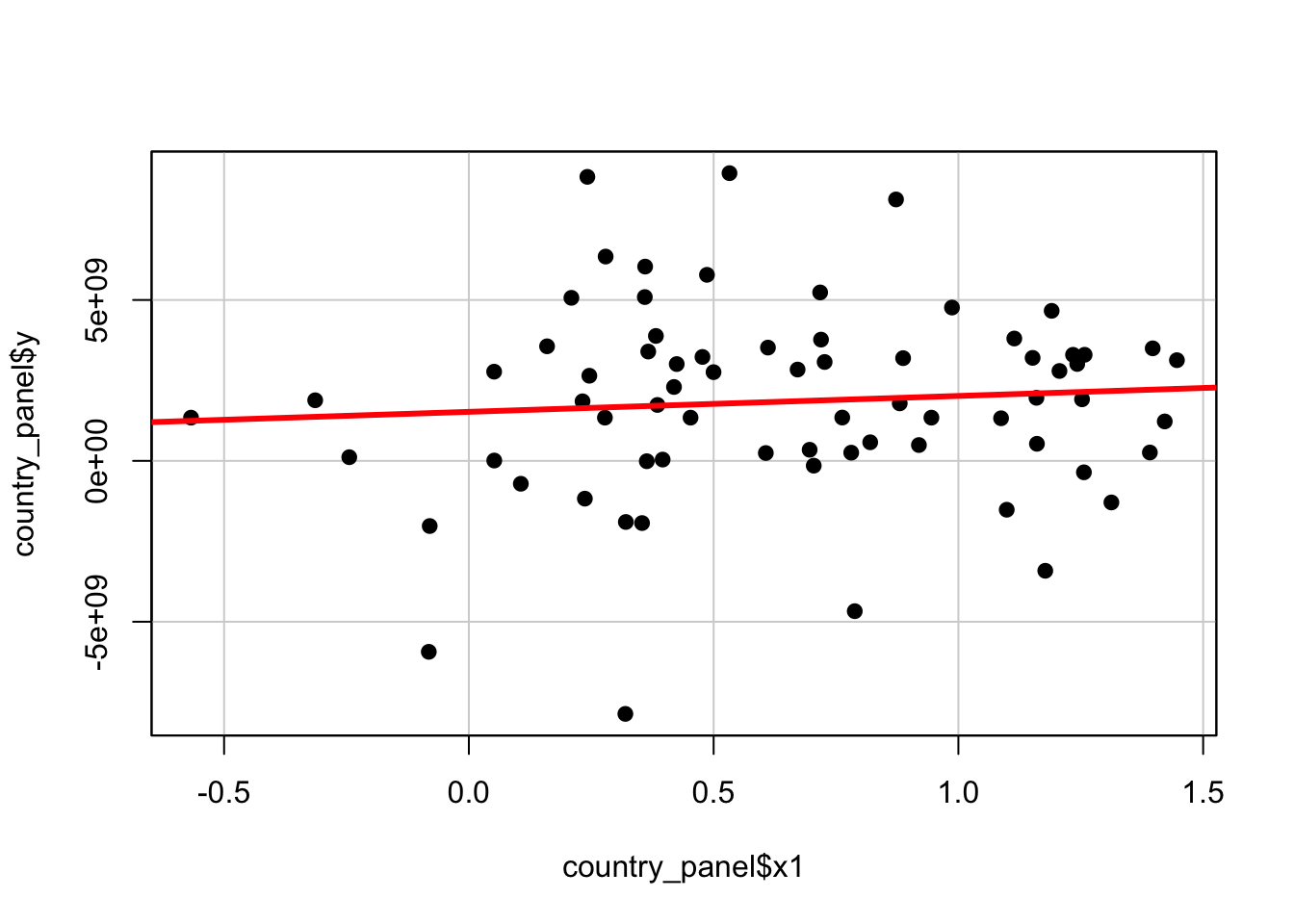
One way of getting around this, and fixing the effects of the country variable, is by using a model incorporating dummy variables through a Least Squares Dummy Variable model (LSDV).
# run a LSDV
fixed_dum <- lm(y ~ x1 + factor(country) - 1, data=country_panel)

# summary
summary(fixed_dum)
##
## Call:
## lm(formula = y ~ x1 + factor(country) - 1, data = country_panel)
##
## Residuals:
## Min 1Q Median 3Q Max
## -8.634e+09 -9.697e+08 5.405e+08 1.386e+09 5.612e+09
##
## Coefficients:
## Estimate Std. Error t value Pr(>|t|)
## x1 2.476e+09 1.107e+09 2.237 0.02889 *
## factor(country)A 8.805e+08 9.618e+08 0.916 0.36347
## factor(country)B -1.058e+09 1.051e+09 -1.006 0.31811
## factor(country)C -1.723e+09 1.632e+09 -1.056 0.29508
## factor(country)D 3.163e+09 9.095e+08 3.478 0.00093 ***
## factor(country)E -6.026e+08 1.064e+09 -0.566 0.57329
## [ reached getOption("max.print") -- omitted 2 rows ]
## ---
## Signif. codes: 0 '***' 0.001 '**' 0.01 '*' 0.05 '.' 0.1 ' ' 1
##
## Residual standard error: 2.796e+09 on 62 degrees of freedom
## Multiple R-squared: 0.4402, Adjusted R-squared: 0.368
## F-statistic: 6.095 on 8 and 62 DF, p-value: 8.892e-06The least square dummy variable model (LSDV) provides a good way to understand fixed effects. By adding the dummy for each country, we are now estimating the pure effect of \(X_{1}\) on \(Y\). Each dummy is absorbing the effects that are particular to each country. Where the independent variable \(X_{1}\) was not significant in the OLS model, after controlling for differences across countries, \(X_{1}\) became significant in the LSDV model. You can clearly see why this is happening in the plot below:
# plot the results
scatterplot(fixed_dum$fitted ~ country_panel$x1|country_panel$country, boxplots=FALSE, smooth=FALSE, col='black')
## Warning in scatterplot.default(X[, 2], X[, 1], groups = X[, 3], xlab = xlab, : number of groups exceeds number of available colors
## colors are recycled# add the LSDV regression lines
abline(lm(y ~ x1, data=country_panel),lwd=3, col='red')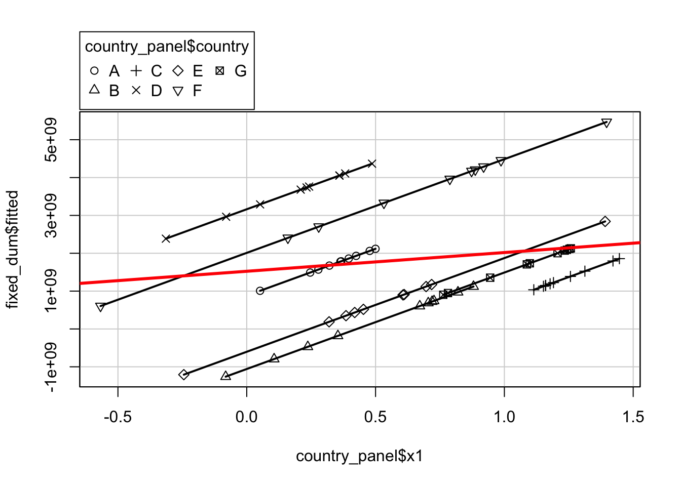
We can also run a country-specific fixed effects model by using specific intercepts for each country. We can achieve this by using the plm package.
# run a fixed effects model
fixed_effects <- plm(y ~ x1, data=country_panel, model='within')

# summary
summary(fixed_effects)
## Oneway (individual) effect Within Model
##
## Call:
## plm(formula = y ~ x1, data = country_panel, model = "within")
##
## Balanced Panel: n = 7, T = 10, N = 70
##
## Residuals:
## Min. 1st Qu. Median Mean 3rd Qu. Max.
## -8.63e+09 -9.70e+08 5.40e+08 0.00e+00 1.39e+09 5.61e+09
##
## Coefficients:
## Estimate Std. Error t-value Pr(>|t|)
## x1 2475617742 1106675596 2.237 0.02889 *
## ---
## Signif. codes: 0 '***' 0.001 '**' 0.01 '*' 0.05 '.' 0.1 ' ' 1
##
## Total Sum of Squares: 5.2364e+20
## Residual Sum of Squares: 4.8454e+20
## R-Squared: 0.074684
## Adj. R-Squared: -0.029788
## F-statistic: 5.00411 on 1 and 62 DF, p-value: 0.028892Here you can check the individual intercepts through fixef(fixed). The coefficient of \(X_{1}\) indicates how much \(Y\) changes on average over time per country: as you can see the results are identical to the results we got from running the LSDV model. Arguably, however, running your model with explicit dummy variables is more informative.
2.3.4 Random effects models
Random effects are the opposite of fixed effects. Contrary to fixed effects, random effects are random and difficult to predict. As such, the effect they will have on a dependent variable \(Y\) is not constant. Think of the cost of renting a one bedroom appartement: rental prices vary greatly depending on location.
If you have reason to believe that differences across entities have some influence on the dependent variable that is not time-dependent, then you would use a random effects model approach over a fixed effects model approach.
# run a random effects model
random_effects <- plm(y ~ x1, data=country_panel, model='random')

# summary
summary(random_effects)
## Oneway (individual) effect Random Effect Model
## (Swamy-Arora's transformation)
##
## Call:
## plm(formula = y ~ x1, data = country_panel, model = "random")
##
## Balanced Panel: n = 7, T = 10, N = 70
##
## Effects:
## var std.dev share
## idiosyncratic 7.815e+18 2.796e+09 0.873
## individual 1.133e+18 1.065e+09 0.127
## theta: 0.3611
##
## Residuals:
## Min. 1st Qu. Median Mean 3rd Qu. Max.
## -8.94e+09 -1.51e+09 2.82e+08 0.00e+00 1.56e+09 6.63e+09
##
## Coefficients:
## Estimate Std. Error z-value Pr(>|z|)
## (Intercept) 1037014329 790626206 1.3116 0.1896
## x1 1247001710 902145599 1.3823 0.1669
##
## Total Sum of Squares: 5.6595e+20
## Residual Sum of Squares: 5.5048e+20
## R-Squared: 0.02733
## Adj. R-Squared: 0.013026
## Chisq: 1.91065 on 1 DF, p-value: 0.16689Interpretation of the coefficients is a little bit tricky since they include both the within-entity and between-entity effects. In this case, the data represents the average effect of \(X_{1}\) over \(Y\) when \(X\) changes across time and between countries by one unit.
If you are not sure whether you should run a fixed effects or a random effects model, you can run a Hausman test to help you with the decision. The Hausman test tests whether the variation across entities (i.e. countries in our example) is uncorrelated with the independent variables. The null hypothesis is that there is no such correlation: if the Hausman specification test comes back significant then it means that you should use a fixed effects model. You run it by comparing the results from both models!
phtest(fixed_effects, random_effects)##
## Hausman Test
##
## data: y ~ x1
## chisq = 3.674, df = 1, p-value = 0.05527
## alternative hypothesis: one model is inconsistentAccording to the Hausman test, we should use the random effects model to estimate the relationship between \(x_1\) and our \(Y\).
Note
Normally, this is not the end of it as there is a sequence of tests that can and should be performed to make sure the model is valid. Testing for hetersokedaticity and stochastic trends, for instance. However, this is out of scope of the current module.
2.4 Take home message
Different models are used for different research questions: the question guides the model. What is important to keep in mind, especially when working with machine learning models, is that not all models are suitable to say something about the relationships between variables. Let alone on whether variable \(X\) is the cause of change in variable \(Y\). In this week’s material, we really wanted to introduce you to some models that do explicitly look at relationships between variables from an econometrics point of view - a very tiny sneak peak if you may. Of course, there are many other advanced econometric models such as models using instrumental variables and difference-in-differences models. Inference is difficult but important in social science, and some of these traditional statistical/econometric method try to get more reliable estimates. What we will be learning in the next couple of weeks will be less interpretable/explanable but it is important to keep some of the issues that came to light during this week’s material in mind. That is it for this week!