7 Spatial-Temporal Mobility Analysis
7.1 Introduction
Against the background of unprecedented growth in private vehicle ownership and the entrenchment of the private car in everyday life, the past decades have seen a growing and ongoing academic and policy debate on how to encourage individuals to change to more sustainable ways of travelling. More recently, researchers have started to build on so-called location-aware technologies, exploring innovative methods to more accurately capture, visualise, and analyse individual spatiotemporal travel patterns: information that can be used to formulate strategies to accommodate the increasing demand for transport vis-à-vis growing environmental and societal concerns.
This week we will be looking at capturing mobility data with Global Positioning Systems. We will further use two types of Machine Learning classifiers, specifically Support Vector Machines and tree-based methods, to classify labeled GPS data into stay and move points. This week is structured around three short videos as well as a tutorial in R with a ‘hands-on’ application of GPS data classification.
Let’s get to it!
Video: Introduction W07
[Lecture slides] [Watch on MS stream]7.1.1 Reading list
Please find the reading list for this week below.
Core reading
- Broach, J. et al.. 2019. Travel mode imputation using GPS and accelerometer data from a multi-day travel survey. Journal of Transport Geography 78: 194-204. [Link]
- Bohte, W. and K. Maat. 2009. Deriving and validating trip purposes and travel modes for multi-day GPS-based travel surveys: A large-scale application in the Netherlands. Transportation Research Part C: Emerging Technologies 17(3): 285–297. [Link]
- Feng, T and H. Timmermans. 2016. Comparison of advanced imputation algorithms for detection of transportation mode and activity episode using GPS data. Transportation Planning and Technology 39(2): 180–194. [Link]
- Nitsche, P. et al.. 2014. Supporting large-scale travel surveys with smartphones - a practical approach. Transportation Research Part C: Emerging Technologies 43: 212–221. [Link]
Supplementary reading
- Behrens, R. et al.. 2006. Collection of passenger travel data in Sub-Saharan African cities: Towards improving survey instruments and procedures. Transport Policy 13: 85-96. [Link]
- Behrens, R. and Del Mistro, R. 2010. Shocking habits: Methodological issues in analyzing changing personal travel behavior over time. International Journal of Sustainable Transportation 4(5): 253-271. [Link]
- Van de Coevering, P. et al.. 2021. Causes and effects between attitudes, the built environment and car kilometres: A longitudinal analysis. Journal of Transport Geography 91: 102982. [Link]
- Van Dijk, J. 2018. Identifying activity-travel points from GPS-data with multiple moving windows. Computers, Environment and Urban Systems 70: 84-101. [Link]
- Wolf, J. 2000. Using GPS data loggers to replace travel diaries in the collection of travel data. Doctoral dissertation. Atlanta, Georgia: Georgia Institute of Technology. [Link]
7.1.2 Technical Help session
Every Thursday between 13h00-14h00 you can join the Technical Help session on Microsoft Teams. The session will be hosted by Alfie. He will be there for the whole hour to answer any question you have live in the meeting or any questions you have formulated beforehand. If you cannot make the meeting, feel free to post the issue you are having in the Technical Help channel on the GEOG0125 Team so that Alfie can help to find a solution.
7.2 GPS data
Mobility is a central aspect of everyday life. In its simplest form, human mobility refers to the movement of individuals from location A to location B. This can be a relocation from one city to another city, as well as a trip from home to work. Transport systems provide the physical nodes and linkages that facilitate this mobility. However, transport systems and road networks in many cities around the world are under pressure as a result of unparalleled growth in private vehicle ownership and increasingly complex and fragmented travel patterns. Particularly in urban areas, this is problematic because it leads to problems such as congestion, accidents, road decay, and reduced accessibility. As such, governments and researchers throughout the world have started to recognise the need to curtail demand for private road transport.
“Technological breakthroughs [alone] are not going to provide the silver bullet for the mitigation of climate change and energy security threats caused by the transport sector” (Stradling and Anable, 2008: 195)
The realisation that increasing road infrastructure and improvements in car technology are not sufficient to address the transport problems around the world has led to the idea that transport planning should shift from supply-side to demand-side passenger transport planning. For this, accurate data are required on individual spatio-temporal behaviour.
Travel data collection methods can roughly be classified into two, not per se mutually exclusive, methods. The first method uses self-reported data, such as data collected through telephone-assisted interviews, computer-assisted interviews, and pen-and-paper interviews. The second method relies on passively collected data, such as data collected through call-detail records and GPS data. Technological developments in the field of location-aware technologies, GPS in particular, have greatly enhanced opportunities to collect accurate data on human spatiotemporal behaviour. GPS data need to be collected and analysed systematically to be intelligible for transport researchers and policy makers. Moreover, the challenges inherent to mobile data collection techniques include not only harnessing the tools to obtain geo-referenced data, but also the development of new skills sets for cleaning, analysing, and interpreting these data.
7.3 GPS data classification
Where GPS technology can precisely register the spatiotemporal elements of activity-travel behaviour, travel characteristics need to be imputed from the data. As such, throughout the last decade or so, a plethora of methods has been developed for identifying trips, activities, and travel modes from raw GPS trajectories. These methods range from deterministic (rule-based) methods to advanced machine learning algorithms. Here, we will focus on using two types of machine learning techniques (Support Vector Machines and tree-based methods) to classify labelled GPS points into stay and move points.
Video: GPS data classification with ML techniques
[Lecture slides] [Watch on MS stream]The segmentation of GPS data into activity and travel episodes is often the first step in a more elaborate process of identifying activity types and transport modes. A major issue with GPS data imputation, however, is the necessity of a ground truth to test whether the imputation algorithm correctly categorises GPS points into activity (stay) points and trips (move) points. We will be using a set of 50 artificially created GPS trajectories that all contain a sequence of stays and moves in Cape Town, South Africa. For the data that we will use, the artificial GPS ‘records’ a measurement every 60 seconds. To further simulate noise in the data, a random sample comprising of 50 per cent of the data points was taken. Besides these raw GPS data, we also have access to a basic road network lay out of the Mother City.
File download
| File | Type | Link |
|---|---|---|
| Cape Town GPS and road data | shp |
Download |
We will start by downloading the files, importing both into R, and looking at what we will be working with. Be careful not to plot the road network file. Because the road network contains around 120,000 individual road segments it will take a long time to draw. Rather have a look at the data in QGIS, which is much more capable of on the fly displaying a large number of features.
# load libraries
library(tidyverse)
library(sf)
library(tmap)

# read gps data
gps <- read_sf('raw/w07/gps_cape_town.shp')

# read road data
road <- read_sf('raw/w07/roads_cape_town.shp')

# inspect
gps
## Simple feature collection with 27019 features and 9 fields
## geometry type: POINT
## dimension: XY
## bbox: xmin: 18.34291 ymin: -34.19419 xmax: 19.06105 ymax: -33.66433
## CRS: 4148
## # A tibble: 27,019 x 10
## stop type duration point_id_n timestamp mode track_id move activity
## <dbl> <chr> <dbl> <dbl> <chr> <chr> <chr> <chr> <chr>
## 1 1 MEDI… 30 1 04/02/19… <NA> 001 STAY STAY
## 2 1 MEDI… 30 2 04/02/19… <NA> 001 STAY STAY
## 3 1 MEDI… 30 5 04/02/19… <NA> 001 STAY STAY
## 4 1 MEDI… 30 9 04/02/19… <NA> 001 STAY STAY
## 5 1 MEDI… 30 10 04/02/19… <NA> 001 STAY STAY
## 6 1 MEDI… 30 12 04/02/19… <NA> 001 STAY STAY
## 7 1 MEDI… 30 14 04/02/19… <NA> 001 STAY STAY
## 8 1 MEDI… 30 16 04/02/19… <NA> 001 STAY STAY
## 9 1 MEDI… 30 18 04/02/19… <NA> 001 STAY STAY
## 10 1 MEDI… 30 22 04/02/19… <NA> 001 STAY STAY
## # … with 27,009 more rows, and 1 more variable: geometry <POINT [°]># inspect
road## Simple feature collection with 125024 features and 1 field
## geometry type: LINESTRING
## dimension: XY
## bbox: xmin: 18.34051 ymin: -34.3001 xmax: 19.12007 ymax: -33.62755
## CRS: 4148
## # A tibble: 125,024 x 2
## id geometry
## <dbl> <LINESTRING [°]>
## 1 1 (18.93353 -34.16301, 18.93345 -34.1631, 18.93335 -34.16318, 18.93…
## 2 2 (18.45615 -34.27366, 18.4545 -34.27321, 18.45298 -34.2728, 18.452…
## 3 3 (18.45615 -34.27366, 18.45674 -34.27201, 18.45683 -34.27181, 18.4…
## 4 4 (18.85612 -34.25045, 18.85621 -34.2506, 18.85633 -34.25087, 18.85…
## 5 5 (19.12007 -34.25944, 19.11977 -34.25952, 19.11936 -34.25961, 19.1…
## 6 6 (18.50105 -33.98948, 18.50102 -33.98942, 18.50105 -33.98935, 18.5…
## 7 7 (18.65381 -34.00991, 18.65355 -34.00979, 18.65251 -34.00931, 18.6…
## 8 8 (18.63738 -34.07209, 18.63846 -34.07193, 18.63924 -34.07183, 18.6…
## 9 9 (18.44389 -34.03779, 18.44389 -34.03798, 18.44388 -34.03826, 18.4…
## 10 10 (18.64958 -34.04498, 18.64729 -34.04547, 18.64228 -34.04652, 18.6…
## # … with 125,014 more rows# inspect
names(gps)## [1] "stop" "type" "duration" "point_id_n" "timestamp"
## [6] "mode" "track_id" "move" "activity" "geometry"# project into Hartbeesthoek94
gps <- gps %>% st_transform(crs='epsg:2053')
road <- road %>% st_transform(crs='epsg:2053')
# plot gps points
tm_shape(gps) +
tm_dots()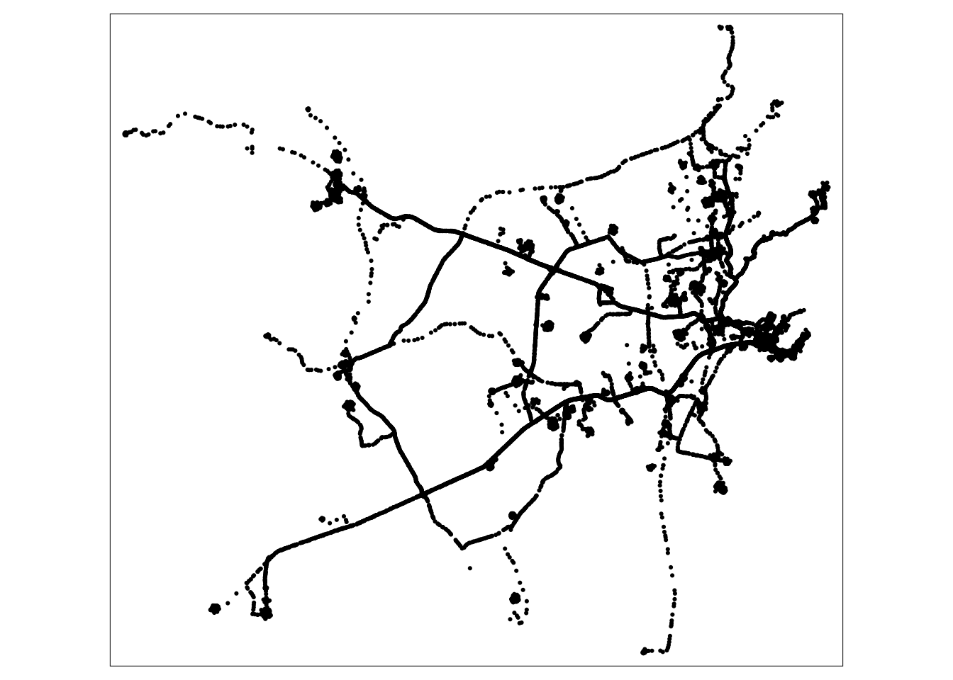
The road network file is relatively simple and only contains road network segments - no additional information (e.g. maximum speed, road type, etc.) is available. The GPS data themselves contain several fields:
| Column heading | Description |
|---|---|
| stop | Stop number within GPS trajectory |
| type | Type of stop (i.e. short, medium, long) |
| duration | Duration of stop in seconds |
| point_id_n | Unique point identifier within GPS trajectory |
| timestamp | Time the point was recorded |
| mode | Travel mode |
| track_id | Unique ID for GPS trajectory |
| move | Whether point is a move or a stay |
| activity | Whether point is a move (including mode) or a stay |
7.3.1 GPS data preparation
The move variable is the variable we will try to predict. Before we split our data into a train and test set, however, we will need to derive some features from our raw GPS data that we can use as our input features: speed, point density, and distance to nearest road segment. As we want to derive information of consecutive measurements, the order of the data is very important right now as the points form a trajectory: so before we calculate anything we start by making sure that the data are ordered correctly: by track_id and timestamp.
# order data so that we do not mix separate trajectories
gps <- gps %>% arrange(track_id,timestamp)

# calculate distance between consecutive points // could take a few minutes
gps <- gps %>%
         group_by(track_id) %>%
         mutate(
                lead_geom = geometry[row_number() + 1],
                dist = st_distance(lead_geom,geometry, by_element=TRUE, which='Euclidean')
                ) %>%
        ungroup()

# inspect
gps
## Simple feature collection with 27019 features and 10 fields
## Active geometry column: geometry
## geometry type: POINT
## dimension: XY
## bbox: xmin: 918250.7 ymin: 3775604 xmax: 986130.2 ymax: 3836086
## CRS: epsg:2053
## # A tibble: 27,019 x 12
## stop type duration point_id_n timestamp mode track_id move activity
## <dbl> <chr> <dbl> <dbl> <chr> <chr> <chr> <chr> <chr>
## 1 1 MEDI… 30 1 04/02/19… <NA> 001 STAY STAY
## 2 1 MEDI… 30 2 04/02/19… <NA> 001 STAY STAY
## 3 1 MEDI… 30 5 04/02/19… <NA> 001 STAY STAY
## 4 1 MEDI… 30 9 04/02/19… <NA> 001 STAY STAY
## 5 1 MEDI… 30 10 04/02/19… <NA> 001 STAY STAY
## 6 1 MEDI… 30 12 04/02/19… <NA> 001 STAY STAY
## 7 1 MEDI… 30 14 04/02/19… <NA> 001 STAY STAY
## 8 1 MEDI… 30 16 04/02/19… <NA> 001 STAY STAY
## 9 1 MEDI… 30 18 04/02/19… <NA> 001 STAY STAY
## 10 1 MEDI… 30 22 04/02/19… <NA> 001 STAY STAY
## # … with 27,009 more rows, and 3 more variables: geometry <POINT [m]>,
## # lead_geom <POINT [m]>, dist [m]# calculate time between consecutive points
gps <- gps %>%
group_by(track_id) %>%
mutate(
lead_time = strptime(timestamp[row_number() + 1], format='%d/%m/%Y %H:%M:%S'),
diff = difftime(lead_time,strptime(timestamp, format='%d/%m/%Y %H:%M:%S'), units='secs')
) %>%
ungroup()
# inspect
gps## Simple feature collection with 27019 features and 12 fields
## Active geometry column: geometry
## geometry type: POINT
## dimension: XY
## bbox: xmin: 918250.7 ymin: 3775604 xmax: 986130.2 ymax: 3836086
## CRS: epsg:2053
## # A tibble: 27,019 x 14
## stop type duration point_id_n timestamp mode track_id move activity
## <dbl> <chr> <dbl> <dbl> <chr> <chr> <chr> <chr> <chr>
## 1 1 MEDI… 30 1 04/02/19… <NA> 001 STAY STAY
## 2 1 MEDI… 30 2 04/02/19… <NA> 001 STAY STAY
## 3 1 MEDI… 30 5 04/02/19… <NA> 001 STAY STAY
## 4 1 MEDI… 30 9 04/02/19… <NA> 001 STAY STAY
## 5 1 MEDI… 30 10 04/02/19… <NA> 001 STAY STAY
## 6 1 MEDI… 30 12 04/02/19… <NA> 001 STAY STAY
## 7 1 MEDI… 30 14 04/02/19… <NA> 001 STAY STAY
## 8 1 MEDI… 30 16 04/02/19… <NA> 001 STAY STAY
## 9 1 MEDI… 30 18 04/02/19… <NA> 001 STAY STAY
## 10 1 MEDI… 30 22 04/02/19… <NA> 001 STAY STAY
## # … with 27,009 more rows, and 5 more variables: geometry <POINT [m]>,
## # lead_geom <POINT [m]>, dist [m], lead_time <dttm>, diff <drtn># calculate speed in kilometres per hour
gps <- gps %>% mutate(speed = as.integer(dist)/as.integer(diff)*3.6)
# inspect
gps## Simple feature collection with 27019 features and 13 fields
## Active geometry column: geometry
## geometry type: POINT
## dimension: XY
## bbox: xmin: 918250.7 ymin: 3775604 xmax: 986130.2 ymax: 3836086
## CRS: epsg:2053
## # A tibble: 27,019 x 15
## stop type duration point_id_n timestamp mode track_id move activity
## * <dbl> <chr> <dbl> <dbl> <chr> <chr> <chr> <chr> <chr>
## 1 1 MEDI… 30 1 04/02/19… <NA> 001 STAY STAY
## 2 1 MEDI… 30 2 04/02/19… <NA> 001 STAY STAY
## 3 1 MEDI… 30 5 04/02/19… <NA> 001 STAY STAY
## 4 1 MEDI… 30 9 04/02/19… <NA> 001 STAY STAY
## 5 1 MEDI… 30 10 04/02/19… <NA> 001 STAY STAY
## 6 1 MEDI… 30 12 04/02/19… <NA> 001 STAY STAY
## 7 1 MEDI… 30 14 04/02/19… <NA> 001 STAY STAY
## 8 1 MEDI… 30 16 04/02/19… <NA> 001 STAY STAY
## 9 1 MEDI… 30 18 04/02/19… <NA> 001 STAY STAY
## 10 1 MEDI… 30 22 04/02/19… <NA> 001 STAY STAY
## # … with 27,009 more rows, and 6 more variables: geometry <POINT [m]>,
## # lead_geom <POINT [m]>, dist [m], lead_time <dttm>, diff <drtn>,
## # speed <dbl>Because we are using consecutive rows to calculate our speed, all of the last measurements within each of the 50 trajectories will not be assigned a value. However, because we do not really want to throw these points out, we will simply assign these points the same speed value as the last point that did get a value assigned.
# fill missing speeds
gps <- gps %>% fill(speed, .direction='down')
Another useful input feature would be a local point density: for each point it would be useful to know how many other points are in its vicinity, for instance, because a clustering of points could be indicative of an activity. Because vicinity is difficult to define, we will use three distance thresholds to create these local point densities: 100m, 250m, and 500m.
# distance thresholds
gps_100m <- st_buffer(gps,100)
gps_250m <- st_buffer(gps,250)
gps_500m <- st_buffer(gps,500)

# loop through trajectories and count the number of points falling within the three distance thresholds
# // this could take a few minutes
df <- gps[0,]
for (t in seq(1,50)) {

        # filter gps trajectory
        gps_sel <- filter(gps, as.integer(track_id)==t)

        # filter buffer
        gps_100m_sel <- filter(gps_100m, as.integer(track_id)==t)
        gps_250m_sel <- filter(gps_250m, as.integer(track_id)==t)
        gps_500m_sel <- filter(gps_500m, as.integer(track_id)==t)

        # intersect
        gps_sel$buf100 <- lengths(st_intersects(gps_sel, gps_100m_sel))
        gps_sel$buf250 <- lengths(st_intersects(gps_sel, gps_250m_sel))
        gps_sel$buf500 <- lengths(st_intersects(gps_sel, gps_500m_sel))

        # bind results
        df <- rbind(df,gps_sel)

}

# rename
gps <- df

# inspect
gps
## Simple feature collection with 27019 features and 16 fields
## Active geometry column: geometry
## geometry type: POINT
## dimension: XY
## bbox: xmin: 918250.7 ymin: 3775604 xmax: 986130.2 ymax: 3836086
## CRS: epsg:2053
## # A tibble: 27,019 x 18
## stop type duration point_id_n timestamp mode track_id move activity
## * <dbl> <chr> <dbl> <dbl> <chr> <chr> <chr> <chr> <chr>
## 1 1 MEDI… 30 1 04/02/19… <NA> 001 STAY STAY
## 2 1 MEDI… 30 2 04/02/19… <NA> 001 STAY STAY
## 3 1 MEDI… 30 5 04/02/19… <NA> 001 STAY STAY
## 4 1 MEDI… 30 9 04/02/19… <NA> 001 STAY STAY
## 5 1 MEDI… 30 10 04/02/19… <NA> 001 STAY STAY
## 6 1 MEDI… 30 12 04/02/19… <NA> 001 STAY STAY
## 7 1 MEDI… 30 14 04/02/19… <NA> 001 STAY STAY
## 8 1 MEDI… 30 16 04/02/19… <NA> 001 STAY STAY
## 9 1 MEDI… 30 18 04/02/19… <NA> 001 STAY STAY
## 10 1 MEDI… 30 22 04/02/19… <NA> 001 STAY STAY
## # … with 27,009 more rows, and 9 more variables: geometry <POINT [m]>,
## # lead_geom <POINT [m]>, dist [m], lead_time <dttm>, diff <drtn>,
## # speed <dbl>, buf100 <int>, buf250 <int>, buf500 <int>Great. We now have a speed variable as well as three local density variables. The last thing we will need to do is for each point calculate the distance to the nearest road segment.
# for each point: get nearest road feature
# // this could take a few minutes
nearest_road <- st_nearest_feature(gps, road)

# for each point: get the distance to the nearest road feature
# // this could take a few minutes
nearest_road_dst <- st_distance(gps, road[nearest_road,], by_element=TRUE, which='Euclidean')

# assign values to gps data set
gps$road_dist <- nearest_road_dst

# inspect
gps
## Simple feature collection with 27019 features and 17 fields
## Active geometry column: geometry
## geometry type: POINT
## dimension: XY
## bbox: xmin: 918250.7 ymin: 3775604 xmax: 986130.2 ymax: 3836086
## CRS: epsg:2053
## # A tibble: 27,019 x 19
## stop type duration point_id_n timestamp mode track_id move activity
## * <dbl> <chr> <dbl> <dbl> <chr> <chr> <chr> <chr> <chr>
## 1 1 MEDI… 30 1 04/02/19… <NA> 001 STAY STAY
## 2 1 MEDI… 30 2 04/02/19… <NA> 001 STAY STAY
## 3 1 MEDI… 30 5 04/02/19… <NA> 001 STAY STAY
## 4 1 MEDI… 30 9 04/02/19… <NA> 001 STAY STAY
## 5 1 MEDI… 30 10 04/02/19… <NA> 001 STAY STAY
## 6 1 MEDI… 30 12 04/02/19… <NA> 001 STAY STAY
## 7 1 MEDI… 30 14 04/02/19… <NA> 001 STAY STAY
## 8 1 MEDI… 30 16 04/02/19… <NA> 001 STAY STAY
## 9 1 MEDI… 30 18 04/02/19… <NA> 001 STAY STAY
## 10 1 MEDI… 30 22 04/02/19… <NA> 001 STAY STAY
## # … with 27,009 more rows, and 10 more variables: geometry <POINT [m]>,
## # lead_geom <POINT [m]>, dist [m], lead_time <dttm>, diff <drtn>,
## # speed <dbl>, buf100 <int>, buf250 <int>, buf500 <int>, road_dist [m]7.3.2 GPS data classification
Now we have added some useful variables to our raw GPS trajectories, we can scale them and move on to our classification algorithms. We will use a C5.0 boosted decision tree, a random forest, and a support vector machine. We will use a test/train split of 70/30.
# libraries
library(e1071)
library(randomForest)
library(C50)
library(caret)

# assign point to train and test
gps <- gps %>% mutate(train = if_else(runif(nrow(gps)) < 0.7, 1, 0))

# create train set, select variables, confirm data types where necessary
gps_train <- gps %>% filter(train==1) %>%
        select(speed,buf100,buf250,buf500,road_dist,move) %>%
        mutate(road_dist=as.numeric(road_dist))

# drop geometry
gps_train <- st_drop_geometry(gps_train)

# scale
gps_train[1:5] <- lapply(gps_train[1:5], function(x) scale(x))

# inspect
gps_train
## # A tibble: 18,943 x 6
## speed[,1] buf100[,1] buf250[,1] buf500[,1] road_dist[,1] move
## <dbl> <dbl> <dbl> <dbl> <dbl> <chr>
## 1 -0.734 -0.474 -0.755 -0.896 -0.742 STAY
## 2 -0.516 -0.452 -0.755 -0.896 -0.240 STAY
## 3 -0.594 -0.563 -0.770 -0.896 -0.316 STAY
## 4 -0.409 -0.519 -0.755 -0.896 0.161 STAY
## 5 -0.450 -0.541 -0.770 -0.896 -0.658 STAY
## 6 -0.622 -0.408 -0.755 -0.896 -0.271 STAY
## 7 -0.560 -0.541 -0.755 -0.896 1.75 STAY
## 8 -0.571 -0.496 -0.755 -0.896 1.05 STAY
## 9 -0.740 -0.474 -0.755 -0.896 -0.533 STAY
## 10 2.49 -0.430 -0.755 -0.896 -0.681 STAY
## # … with 18,933 more rows# create train set, select variables, confirm data types where necessary
gps_test <- gps %>% filter(train==0) %>%
select(speed,buf100,buf250,buf500,road_dist,move) %>%
mutate(road_dist=as.numeric(road_dist))
# drop geometry
gps_test <- st_drop_geometry(gps_test)
# scale
gps_test[1:5] <- lapply(gps_test[1:5], function(x) scale(x))
# inspect
gps_test## # A tibble: 8,076 x 6
## speed[,1] buf100[,1] buf250[,1] buf500[,1] road_dist[,1] move
## <dbl> <dbl> <dbl> <dbl> <dbl> <chr>
## 1 -0.682 -0.501 -0.760 -0.902 -0.241 STAY
## 2 -0.586 -0.567 -0.760 -0.902 1.44 STAY
## 3 -0.641 -0.478 -0.760 -0.902 -0.209 STAY
## 4 4.83 -0.612 -0.938 -1.04 -0.547 MOVE
## 5 5.22 -0.589 -0.923 -1.03 -0.391 MOVE
## 6 4.83 -0.612 -0.938 -1.04 -0.698 MOVE
## 7 5.37 -0.612 -0.938 -1.04 -0.408 MOVE
## 8 -0.714 -0.545 -0.686 -0.772 -0.625 STAY
## 9 -0.722 -0.434 -0.597 -0.772 0.563 STAY
## 10 -0.467 -0.301 -0.597 -0.772 0.475 STAY
## # … with 8,066 more rowsLet’s train our models on our train data and directly predict on our test data.
# boosted decision tree with 5 boosting iterations
train_boost <- C5.0(as.factor(move) ~., data=gps_train, trials=5)

# support vector machine
train_svm <- svm(as.factor(move) ~ ., data=gps_train)

# random forest with 500 trees, 3 variables at each split, sampling with replacement
train_rf <- randomForest(as.factor(move) ~ ., data=gps_train, ntree=500, replace=TRUE, mtry=3)

# predict boosted decision tree
test_boost <- predict(train_boost, gps_test)

# predict support vector machine
test_svm <- predict(train_svm, gps_test)

# predict random forest
test_rf <- predict(train_rf, gps_test)
We will use a confusion matrix to inspect our results. A confusion matrix is a table that is often used to describe the performance of a classification model on a set of test data for which the actual values are known. In other words, a confusion matrix can be used to compare the predictions our models make to the ground truth. A confusion matrix basically informs you for all prediction classes how many data points where predicted correctly and how many data points were predicted incorrectly.
# create confusion matrices
matrix_boost <-table(test_boost, gps_test$move)
matrix_svm <- table(test_svm, gps_test$move)
matrix_rf <- table(test_rf, gps_test$move)

# inspect
matrix_boost
##
## test_boost MOVE STAY
## MOVE 3175 128
## STAY 125 4648# inspect
matrix_svm##
## test_svm MOVE STAY
## MOVE 3184 158
## STAY 116 4618# inspect
matrix_rf##
## test_rf MOVE STAY
## MOVE 3155 77
## STAY 145 4699# get overall accuracy boosted decision tree
confusionMatrix(matrix_boost)$overall## Accuracy Kappa AccuracyLower AccuracyUpper AccuracyNull
## 0.9686726 0.9351892 0.9646383 0.9723639 0.5913819
## AccuracyPValue McnemarPValue
## 0.0000000 0.8999386# get overall accuracy support vector machine
confusionMatrix(matrix_svm)$overall## Accuracy Kappa AccuracyLower AccuracyUpper AccuracyNull
## 0.96607231 0.92993754 0.96188997 0.96991376 0.59138187
## AccuracyPValue McnemarPValue
## 0.00000000 0.01325288# get overall accuracy random forest
confusionMatrix(matrix_rf)$overall## Accuracy Kappa AccuracyLower AccuracyUpper AccuracyNull
## 9.725111e-01 9.429407e-01 9.687083e-01 9.759677e-01 5.913819e-01
## AccuracyPValue McnemarPValue
## 0.000000e+00 6.900148e-06As we can see, all algorithms are highly accurate in classifying our artificial GPS points into moves and stays using the input features that were derived from the raw GPS trajectory data.
7.3.3 Exercise
Now we have worked through classifying our points into moves and stays using raw GPS points, there are three further exercises that we want you to do:
- Add a new set of variables that, for every point in the dataset, contains the number of points within a distance of 100m, 250m, and 500m but for only those points that are within 5 minutes (both sides) of the point under consideration (i.e. use a moving time window to select the points that qualify). So, for instance, for point \(x\) 10 other points are within a distance of 100m but only 5 of these points were recorded within 5 minutes of point \(x\): we now only want those 5 points and not the full 10 points. Please note: this is not a trivial task and you will have to considerably change the code that you have used so far.
- Instead of using the move column, use the activity column to classify the GPS points into travel modes (i.e. walk, bike , car) and stays. Incorporate all existing variables as well as the three variables you created in Exercise 1.
- Assess the relative importance of each of the input variables used in Exercise 2 by permutating (that is shuffling) each input variable and re-running the train and test sequence. So, for instance, shuffle the values within the speed column but leaving all the other values untouched, train the three models, and look at the accuracy and Kappa values to see the new results. Repeat this process for all columns in which every time one of the columns gets permutated but all the other values are untouched. With every iteration you save the accuracy and Kappa values so to get an idea about each variable’s relative importance: the variable that causes the largest drop in accuracy and Kappa values is relatively the most important one.
Tip 1: You can shuffle your data by sampling without replacement, e.g.gps_test$speed <- sample(gps_test$speed).
Tip 2: Create a function or a loop to conduct this process!
7.4 Take home message
Where GPS technology can precisely register locational information, travel characteristics need to be imputed from the data before it can be used by transport researchers and policy makers. As such, throughout the last decade, various methods have been developed for identifying trips, activities, and travel modes from raw GPS trajectories. In this week’s material, we took a closer look at GPS data. We also introduced you to three different discriminative classifiers to classify GPS points into moves and stays. Be aware that we only given you a brief introduction to these classifiers here and there are in fact many different implementations of decision trees as well many ways of parameterising support vector machines (e.g. choice of kernel). It is also important to keep in mind that because the GPS points used in the tutorial were artificially created, the models results in relatively high prediction rates and will be very difficult to transfer to a different context. While this is obviously an issue, the advantage of using artificial data is that parameters and noise levels can be precisely tuned which allow you to systematically compare, test, and develop different algorithms.
7.5 Attributions
This week’s content and practical uses content and inspiration from:
- Van Dijk, J. 2017. Designing Travel Behaviour Change Interventions: a spatiotemporal perspective. Doctoral dissertation. Stellenbosch: Stellenbosch University. [Link]
- Van Dijk, J. 2018. Identifying activity-travel points from GPS-data with multiple moving windows. Computers, Environment and Urban Systems 70: 84-101. [Link]