2 Spatial autocorrelation
2.1 This week
This week, we focus on the first of two key properties of spatial data: spatial dependence. Spatial dependence is the idea that the observed value of a variable in one location is often dependent (to some degree) on the observed value of the same value in a nearby location. For spatial analysis, this dependence can be assessed and measured statistically by considering the level of spatial autocorrelation between values of a specific variable, observed in either different locations or between pairs of variables observed at the same location. Spatial autocorrelation occurs when these values are not independent of one another and instead cluster together across geographic space.
A critical first step of spatial autocorrelation is to define the criteria under which a spatial unit (e.g. an areal or point unit) can be understood as a “neighbour” to another unit. As highlighted in previous weeks, spatial properties can often take on several meanings, and as a result, have an impact on the validity and accuracy of spatial analysis. This multiplicity also can be applied to the concept of spatial neighbours which can be defined through adjacency, contiguity or distance-based measures. As the specification of these criteria can impact the results, the definition followed therefore need to be grounded in particular theory that aims to represent the process and variable investigated.
2.2 Lecture recording
2.3 Reading list
- Gimond, M. 2021. Intro to GIS and spatial analysis. Chapter 13: Spatial autocorrelation. [Link]
- Longley, P. et al. 2015. Geographic Information Science & systems, Chapter 2: The Nature of Geographic Data. [Link]
- Longley, P. et al. 2015. Geographic Information Science & systems, Chapter 13: Spatial Analysis. [Link]
- Radil, S. 2016. Spatial analysis of crime. In: Huebner, B. and Bynum, T. The Handbook of Measurement Issues in Criminology and Criminal Justice, Chapter 24, pp.536-554. [Link]
2.4 Case study
This week looks at spatial dependence and autocorrelation in detail, focusing on the different methods of assessment. As part of this, we look at the multiple methods to defining spatial neighbours and their suitability of use across different spatial phenomena – and how this approach is used to generate spatial weights for use within these spatial autocorrelation methods as well as their potential to generate spatially-explicit variables.
We put these learnings into practice through an analysis of spatial dependence of areal crime data, experimenting with the deployment of different neighbours and the impact of their analyses. For this practical we will look at the distribution of thefts from persons in the borough of Camden.
2.5 Neighbours
If we want to come up with quantifiable descriptions of variables and how they vary over space, then we need to find ways of quantifying the distance from point to point. When you attach values to the polygons of wards in London, and visualise them, different patterns appear, and the different shapes and sizes of the polygons effect what these patterns look like. There can appear to be clusters, or the distribution can be random. If you want to explain and discuss variables, the underlying causes, and the possible solutions to issues, it becomes useful to quantify how clustered, or at the opposite end, how random these distributions are. This issue is known as spatial autocorrelation.
In raster data, variables are measured at regular spatial intervals (or interpolated to be represented as such). Each measurement is regularly spaced from its neighbours, like the pixels on the screen you are reading this from. With vector data, the distance of measurement to measurement, and the size and shape of the “pixel” of measurement becomes part of the captured information. Whilst this can allow for more nuanced representations of spatial phenomena, it also means that the quantity and type of distance between measurements needs to be acknowledged.
If you want to calculate the relative spatial relation of distributions, knowledge of what counts as a “neighbour” becomes useful. Neighbours can be neighbours due to euclidean distance (distance in space), or they can be due to shared relationships, like a shared boundary, or they can simply be the nearest neighbour, if there aren’t many other vectors around. Depending on the variable you are measuring the appropriateness of neighbourhood calculation techniques can change.
2.6 Getting started
To begin let’s load the libraries needed for this practical. Install the libraries where necessary.
# libraries
library(sf)
library(nngeo)
library(data.table)
library(tmap)
library(tidyverse)
Download the data necessary for the practical and put it in a folder we can find. We will use the same structure as the data directory from the previous week. If you are using the same directory for this weeks work then you can put these files in the same directories. If not make new ones with names that work. Alternatively you can make your own structure and use that.
Note
To follow along with the code as it is and not edit the file paths there should be a folder called data/ in your project working directory, if not best to make one. Inside this create a folder called crime. Put the 2019_camden_theft_from_person.csv file in that folder. Inside your data/ directory there should already be a folder called administrative_boundaries. Save the files belonging to the OAs_camden_2011.shp in here.
File download
| File | Type | Link |
|---|---|---|
| Theft in Camden | shp, csv |
Download |
2.7 Loading our data sets
Now we have the data in the correct folders, we can load and plot the shape data.
# load camden boundaries
camden_oas <- st_read('data/administrative_boundaries/OAs_camden_2011.shp', crs=27700)
## Reading layer `OAs_camden_2011' from data source
## `/Users/justinvandijk/Dropbox/UCL/Web/jtvandijk.github.io/GEOG0114_21_22/data/administrative_boundaries/OAs_camden_2011.shp'
## using driver `ESRI Shapefile'
## Simple feature collection with 749 features and 17 fields
## Geometry type: MULTIPOLYGON
## Dimension: XY
## Bounding box: xmin: 523954.5 ymin: 180965.4 xmax: 531554.9 ymax: 187603.6
## Projected CRS: OSGB 1936 / British National Grid# inspect
tm_shape(camden_oas) +
tm_polygons()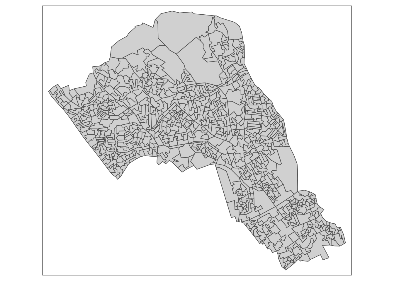
You can see how one of these output areas could have many more neighbours than others, they vary a great deal in size and shape. The dimensions of these objects change over space, as a result the measurements within them must change too.
Output areas are designed to convey and contain census information, so they are created in a way that maintains a similar number of residents in each one. The more sparsely populated an OA the larger it is. Output Areas are designed to cover the entirety of the land of England and Wales so they stretch over places where there are no people. In the north of Camden the largest Ouput Areas span over Hampstead Heath, a large park.
Let’s explore how to find different kinds of neighbours using the example of one ‘randomly’ selected output area (E00004174) that happens to contain the UCL main campus.
# highlight E00004174
tm_shape(camden_oas) +
tm_borders(col='black') +
tm_shape(camden_oas[camden_oas$OA11CD=='E00004174',]) +
tm_fill(col='red')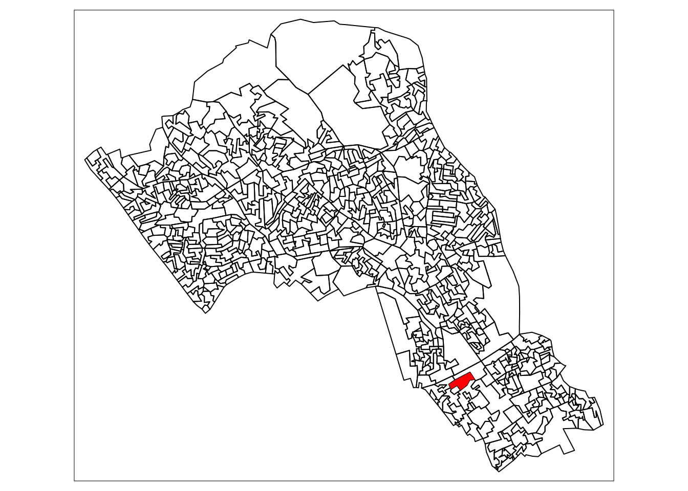
2.8 Euclidean neighbours
The first way we are going to call something a neighbour is by using Euclidean distance. As our OA shapefile is projected in BNG (British National Grid), the coordinates are planar, going up 1 is the same distance as going sideways 1. Even better the coordinates are in metric measurements so it’s easy to make up heuristic distances.
Let’s call every output area with a centroid 500m or less away from the centroid of our chosen OA a neighbour:
- we select only the the centroid of our chosen output area and all other areas (with
st_centroid()) - we set the maximum number of neighbours we want to find to “50” (with parameter
k) - we set the maximum distance of calling an OA centroid a neigbour to “500” (with parameter
maxdist) - we return a sparse matrix that tells us whether each OA is a neighbour or not (with parameter
sparse)
# assign our chosen OA to a variable
chosen_oa <- 'E00004174'
# identify neighbours
chosen_oa_neighbours <- st_nn(st_geometry(st_centroid(camden_oas[camden_oas$OA11CD==chosen_oa,])),
st_geometry(st_centroid(camden_oas)),
sparse = TRUE,
k = 50,
maxdist = 500) ## projected points# inspect
class(chosen_oa_neighbours)## [1] "list"# get the names (codes) of these neighbours
neighbour_names <- camden_oas[chosen_oa_neighbours[[1]],]
neighbour_names <- neighbour_names$OA11CD
# inspect
tm_shape(camden_oas) +
tm_borders() +
# highlight only the neighbours
tm_shape(camden_oas[camden_oas$OA11CD %in% neighbour_names,]) +
tm_fill(col = 'green') +
# highlight only the chosen OA
tm_shape(camden_oas[camden_oas$OA11CD==chosen_oa,]) +
tm_fill(col = 'red') +
tm_shape(camden_oas) +
# overlay the borders
tm_borders(col='black')
2.9 Shared boundary neighbours
The next way of calculating neighbours takes into account the actual shape and location of the polygons in our shapefile. This has only recently been added to the world of sf(), previously we would have reverted to using the sp() package and others that depend on it such as spdep().
We can create two functions that check whether any polygons share boundaries or overlap one another, and then also check by how much. These new functions are based on the st_relate() function. The different cases of these are known as queen, and rook. These describe the relations in a similar way to the possible chess board movements of these pieces.
Note
Do have a look at the short lectures by Luc Anselin on Moran’s I, the interpretation of Moran’s I, and neighbours and spatial weights for some additional explanation on measuring spatial autocorrelation with Moran’s I.
# for rook case
st_rook = function(a, b = a) st_relate(a, b, pattern = 'F***1****')
# for queen case
st_queen <- function(a, b = a) st_relate(a, b, pattern = 'F***T****')Now that we’ve created the functions lets try them out.
# identify neighbours
chosen_oa_neighbours <- st_rook(st_geometry(camden_oas[camden_oas$OA11CD==chosen_oa,]),
st_geometry(camden_oas))
# get the names (codes) of these neighbours
neighbour_names <- camden_oas[chosen_oa_neighbours[[1]],]
neighbour_names <- neighbour_names$OA11CD
# inspect
tm_shape(camden_oas) +
tm_borders() +
# highlight only the neighbours
tm_shape(camden_oas[camden_oas$OA11CD %in% neighbour_names,]) +
tm_fill(col = 'green') +
tm_shape(camden_oas[camden_oas$OA11CD==chosen_oa,]) +
# highlight only the chosen OA
tm_fill(col = 'red') +
tm_shape(camden_oas) +
# overlay the borders
tm_borders(col='black')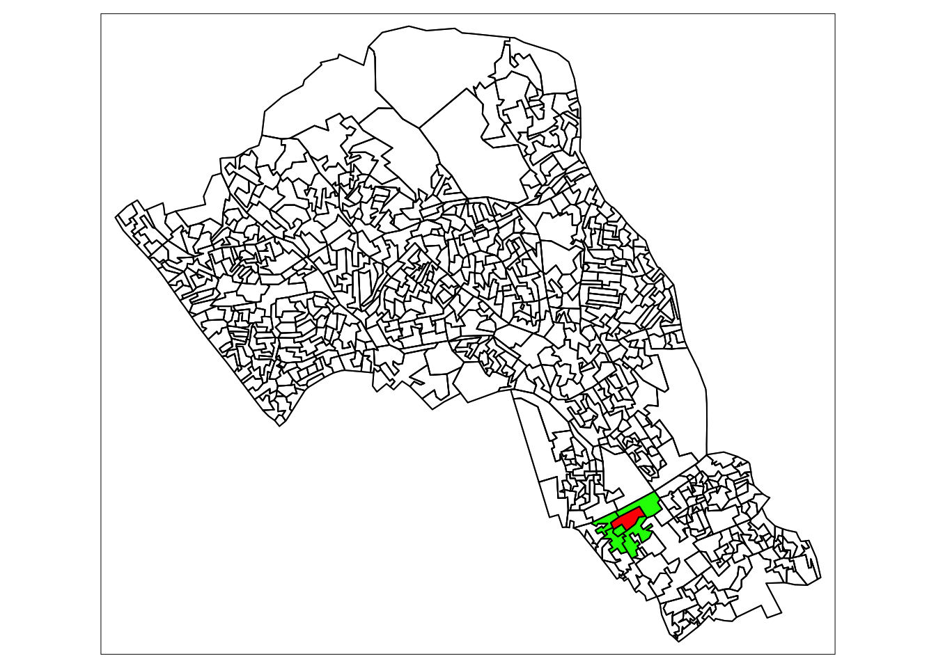
Note
Because the tolerance of the shared boundaries in the st_rook() pattern and the st_queen() pattern, in this example they both assign the same neighbours. This is true for many non-square polygons as the difference is often given as whether two shapes share one or more points. Therefore the difference can have more to do with the resolution and alignment of your polygons than the actual spatial properties they represent. They can and do find different neighbours in other situations. Follow the grid example in the st_relate() documentation if you want to see it working.
2.10 Theft in Camden
Now that we have found the different ways of finding neighbours we can consider how they relate to one another. There are two ways of looking at spatial autocorrelation:
- Global: This is a way of creating a metric of how regularly or irregularly clustered the variables are over the entire area studied.
- Local: This is the difference between an area and its neighbours. You would expect neighbours to be similar, but you can find exceptional places and results by seeing if places are quantifiably more like or dislike their neighbours than the average other place.
But before we start that let’s get into the data we are going to use! We’ll be using personal theft data from around Camden. Our neighbourhood analysis of spatial autocorrelation should allow us to quantify the pattern of distribution of reported theft from persons in Camden in 2019.
# load theft data
camden_theft <- fread('data/crime/2019_camden_theft_from_person.csv')
# convert csv to sf object
camden_theft <- st_as_sf(camden_theft, coords = c('X','Y'), crs = 27700)
# inspect
tm_shape(camden_oas) +
tm_polygons() +
tm_shape(camden_theft) +
tm_dots()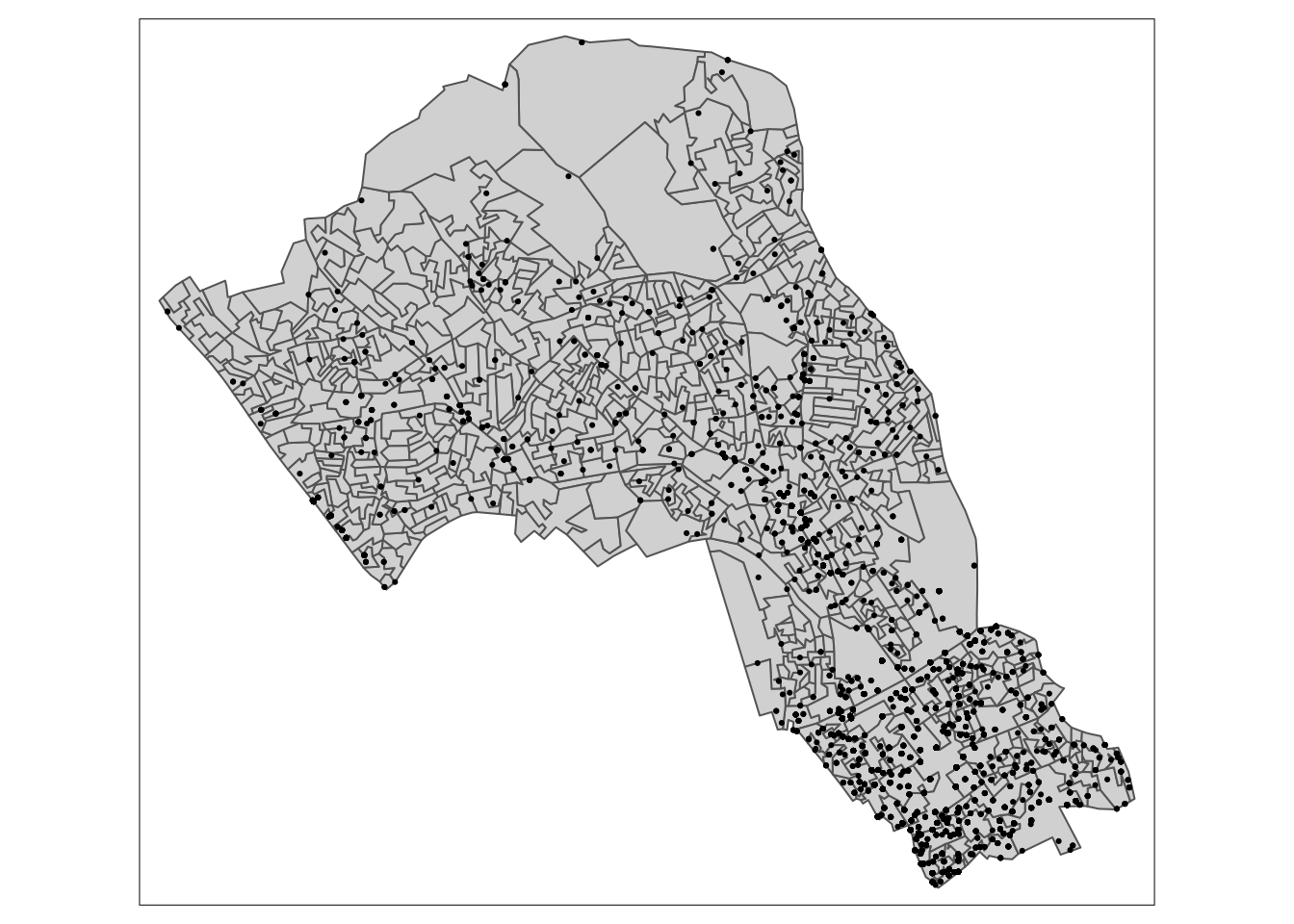
This is point data, but we are interested in the polygons and how this data relates to the administrative boundaries it is within. Let’s count the number of thefts in each OA. This is a spatial operation that is often called “point in polygon”. As we are just counting the number of occurrences in each polygon it is quite easy. In the future you may often want to aggregate over points for an area, or in reverse assign values from the polygon to the points.
# thefts in camden
camden_oas$n_thefts <- lengths(st_intersects(camden_oas, camden_theft))

# inspect
tm_shape(camden_oas) +
  tm_fill(col='n_thefts')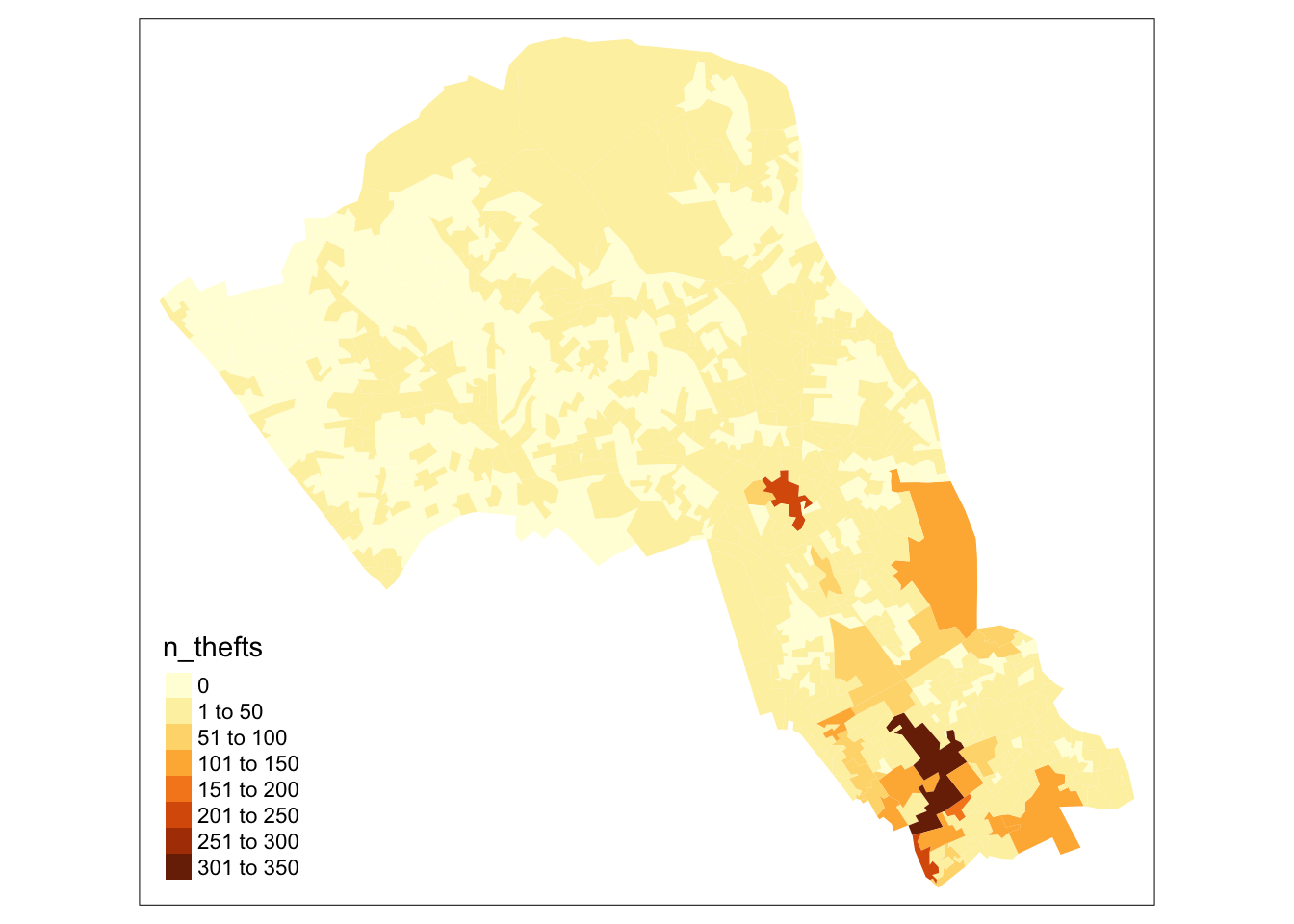
You can see our map isskewed by central London, meaning that the results in central London (the south of Camden) are so much larger than those in the north that it makes it harder to see the smaller differences between other areas. We’ll take the square root of the number of thefts to remedy this.
# square root of thefts
camden_oas$sqrt_n_thefts <- sqrt(camden_oas$n_thefts)

# inspect
tm_shape(camden_oas) +
  tm_fill(col='sqrt_n_thefts')
There: a slightly more nuanced picture
2.11 Global Moran’s I
With a Global Moran’s I we can test how “random” the spatial distribution of these values is. Global Moran’s I is a metric between -1 and 1. -1 is a completely even spatial distribution of values, 0 is a “random” distribution, and 1 is a “non-random” distribution of clearly defined clusters.
To calculate the Global Moran’s I you need an adjacency matrix that contains the information of whether or not an OA is next to another. For an even more nuanced view you can include distance, or a distance weighting in the matrix rather than just the TRUE or FALSE, to take into account the strength of the neighbourhoodness. Because of the way Moran’s I functions in R it is necessary to use the sp and spdep libraries. So load them in.
# libraries
library(sp)
library(spdep)
## Loading required package: spDataAs you will see these methods and functions have quite esoteric and complicated syntax. Some of the operations they will do will be similar to the examples shown earlier, but the way they assign and store variables makes it much quicker to run complex spatial operations.
# inspect
class(camden_oas)
## [1] "sf" "data.frame"# convert to sp
camden_oas_sp <- as_Spatial(camden_oas, IDs=camden_oas$OA11CD)
# inspect
class(camden_oas_sp)## [1] "SpatialPolygonsDataFrame"
## attr(,"package")
## [1] "sp"Now we can make the esoteric and timesaving “nb” object in which we store for each OA which other OAs are considered to be neighbours.
# create an nb object
camden_oas_nb <- poly2nb(camden_oas_sp, row.names=camden_oas_sp$OA11CD)

# inspect
class(camden_oas_nb)
## [1] "nb"# inspect
str(camden_oas_nb,list.len=10)## List of 749
## $ : int [1:7] 10 15 215 303 327 375 464
## $ : int [1:5] 19 72 309 365 430
## $ : int [1:3] 133 152 709
## $ : int [1:7] 78 131 152 286 314 582 651
## $ : int [1:5] 67 316 486 492 703
## $ : int [1:8] 7 68 317 487 556 612 625 638
## $ : int [1:3] 6 68 317
## $ : int [1:7] 57 58 164 358 429 605 684
## $ : int [1:5] 58 164 489 609 700
## $ : int [1:7] 1 215 245 311 327 366 644
## [list output truncated]
## - attr(*, "class")= chr "nb"
## - attr(*, "region.id")= chr [1:749] "E00004395" "E00004314" "E00004578" "E00004579" ...
## - attr(*, "call")= language poly2nb(pl = camden_oas_sp, row.names = camden_oas_sp$OA11CD)
## - attr(*, "type")= chr "queen"
## - attr(*, "sym")= logi TRUENext, we need to assign weights to each neighbouring polygon. In our case, each neighbouring polygon will be assigned equal weight with style='W'. After this, we can calculate a value for the Global Moran’s I.
# create the list weights object
nb_weights_list <- nb2listw(camden_oas_nb, style='W')

# inspect
class(nb_weights_list)
## [1] "listw" "nb"# Moran's I
mi_value <- moran(camden_oas_sp$n_thefts,nb_weights_list,n=length(nb_weights_list$neighbours),S0=Szero(nb_weights_list))
# inspect
mi_value## $I
## [1] 0.4772137
##
## $K
## [1] 75.21583The Global Moran’s I seems to indicate that there is indeed some spatial autocorrelation in our data, however, this is just a quick way to check the score. To do so properly we need to compare our score a randomly distributed version of the variables. We can do this by using something called a Monte Carlo simulation.
# run a Monte Carlo simulation 599 times
mc_model <- moran.mc(camden_oas_sp$n_thefts, nb_weights_list, nsim=599)

# inspect
mc_model
##
## Monte-Carlo simulation of Moran I
##
## data: camden_oas_sp$n_thefts
## weights: nb_weights_list
## number of simulations + 1: 600
##
## statistic = 0.47721, observed rank = 600, p-value = 0.001667
## alternative hypothesis: greaterThis model shows that our distribution of thefts differs significantly from a random distribution. As such, we can conclude that there is significant spatial autocorrelation in our theft data set.
2.12 Local Moran’s I
With a measurement of local spatial autocorrelation we could find hotspots of theft that are surrounded by areas of much lower theft. According to the previous global statistic these are not randomly distributed pockets but would be outliers against the general trend of clusteredness! These could be areas that contain very specific locations, where interventions could be made that drastically reduce the rate of crime rather than other areas where there is a high level of ambient crime.
# create an nb object
camden_oas_nb <- poly2nb(camden_oas_sp, row.names=camden_oas_sp$OA11CD)

# create the list weights object
nb_weights_list <- nb2listw(camden_oas_nb, style='W')

# Local Moran's I
local_moran_camden_oa_theft <- localmoran(camden_oas_sp$n_thefts, nb_weights_list)
To properly utilise these local statistics and make an intuitively useful map, we need to combine them with our crime count variable. Because of the way the new variable will be calculated, we first need to rescale our variable so that the mean is 0.
# rescale
camden_oas_sp$scale_n_thefts <- scale(camden_oas_sp$n_thefts)
To compare this rescaled value against its neighbours, we subsequently need to create a new column that carries information about the neighbours. This is called a spatial lag function. The “lag” just refers to the fact you are comparing one observation against another, this can also be used between timed observations. In this case, the “lag” we are looking at is between neighbours.
# create a spatial lag variable
camden_oas_sp$lag_scale_n_thefts <- lag.listw(nb_weights_list, camden_oas_sp$scale_n_thefts)
Now we have used sp for all it is worth it’s time to head back to the safety of sf() before exploring any forms of more localised patterns.
# convert to sf
camden_oas_moran_stats <- st_as_sf(camden_oas_sp)
To make a human readable version of the map we will generate some labels for our findings from the Local Moran’s I stats. This process calculates what the value of each polygon is compared to its neighbours and works out if they are similar or dissimilar and in which way, then gives them a text label to describe the relationship.
# set a significance value
sig_level <- 0.1

# classification with significance value
camden_oas_moran_stats$quad_sig <- ifelse(camden_oas_moran_stats$scale_n_thefts > 0 &
                                          camden_oas_moran_stats$lag_scale_n_thefts > 0 &
                                          local_moran_camden_oa_theft[,5] <= sig_level,
                                          'high-high',
                                   ifelse(camden_oas_moran_stats$scale_n_thefts <= 0 &
                                          camden_oas_moran_stats$lag_scale_n_thefts <= 0 &
                                          local_moran_camden_oa_theft[,5] <= sig_level,
                                          'low-low',
                                   ifelse(camden_oas_moran_stats$scale_n_thefts > 0 &
                                          camden_oas_moran_stats$lag_scale_n_thefts <= 0 &
                                          local_moran_camden_oa_theft[,5] <= sig_level,
                                          'high-low',
                                   ifelse(camden_oas_moran_stats$scale_n_thefts <= 0 &
                                          camden_oas_moran_stats$lag_scale_n_thefts > 0 &
                                          local_moran_camden_oa_theft[,5] <= sig_level,
                                          'low-high',
                                   ifelse(local_moran_camden_oa_theft[,5] > sig_level,
                                          'not-significant',
                                          'not-significant')))))

# classification without significance value
camden_oas_moran_stats$quad_non_sig <- ifelse(camden_oas_moran_stats$scale_n_thefts > 0 &
                                              camden_oas_moran_stats$lag_scale_n_thefts > 0,
                                              'high-high',
                                       ifelse(camden_oas_moran_stats$scale_n_thefts <= 0 &
                                              camden_oas_moran_stats$lag_scale_n_thefts <= 0,
                                              'low-low',
                                       ifelse(camden_oas_moran_stats$scale_n_thefts > 0 &
                                              camden_oas_moran_stats$lag_scale_n_thefts <= 0,
                                              'high-low',
                                       ifelse(camden_oas_moran_stats$scale_n_thefts <= 0 &
                                              camden_oas_moran_stats$lag_scale_n_thefts > 0,
                                              'low-high',NA))))
To understand how this is working we can look at the data non-spatially. As we rescaled the data, our axes should split the data neatly into their different area vs spatial lag relationship categories. Let’s make the scatterplot using the scaled number of thefts for the areas in the x axis and their spatially lagged results in the y axis.
# plot the results without the statistical significance
ggplot(camden_oas_moran_stats, aes(x = scale_n_thefts,
                                   y = lag_scale_n_thefts,
                                   color = quad_non_sig)) +
  geom_vline(xintercept = 0) + # plot vertical line
  geom_hline(yintercept = 0) + # plot horizontal line
  xlab('Scaled Thefts (n)') +
  ylab('Lagged Scaled Thefts (n)') +
  labs(colour='Relative to neighbours') +
  geom_point()
# plot the results with the statistical significance
ggplot(camden_oas_moran_stats, aes(x = scale_n_thefts,
                                   y = lag_scale_n_thefts,
                                   color = quad_sig)) +
  geom_vline(xintercept = 0) + # plot vertical line
  geom_hline(yintercept = 0) + # plot horizontal line
  xlab('Scaled Thefts (n)') +
  ylab('Lagged Scaled Thefts (n)') +
  labs(colour='Relative to neighbours') +
  geom_point()
Now let’s see how they are arranged spatially.
# map all of the results here
tm_shape(camden_oas_moran_stats) +
  tm_fill(col = 'quad_non_sig')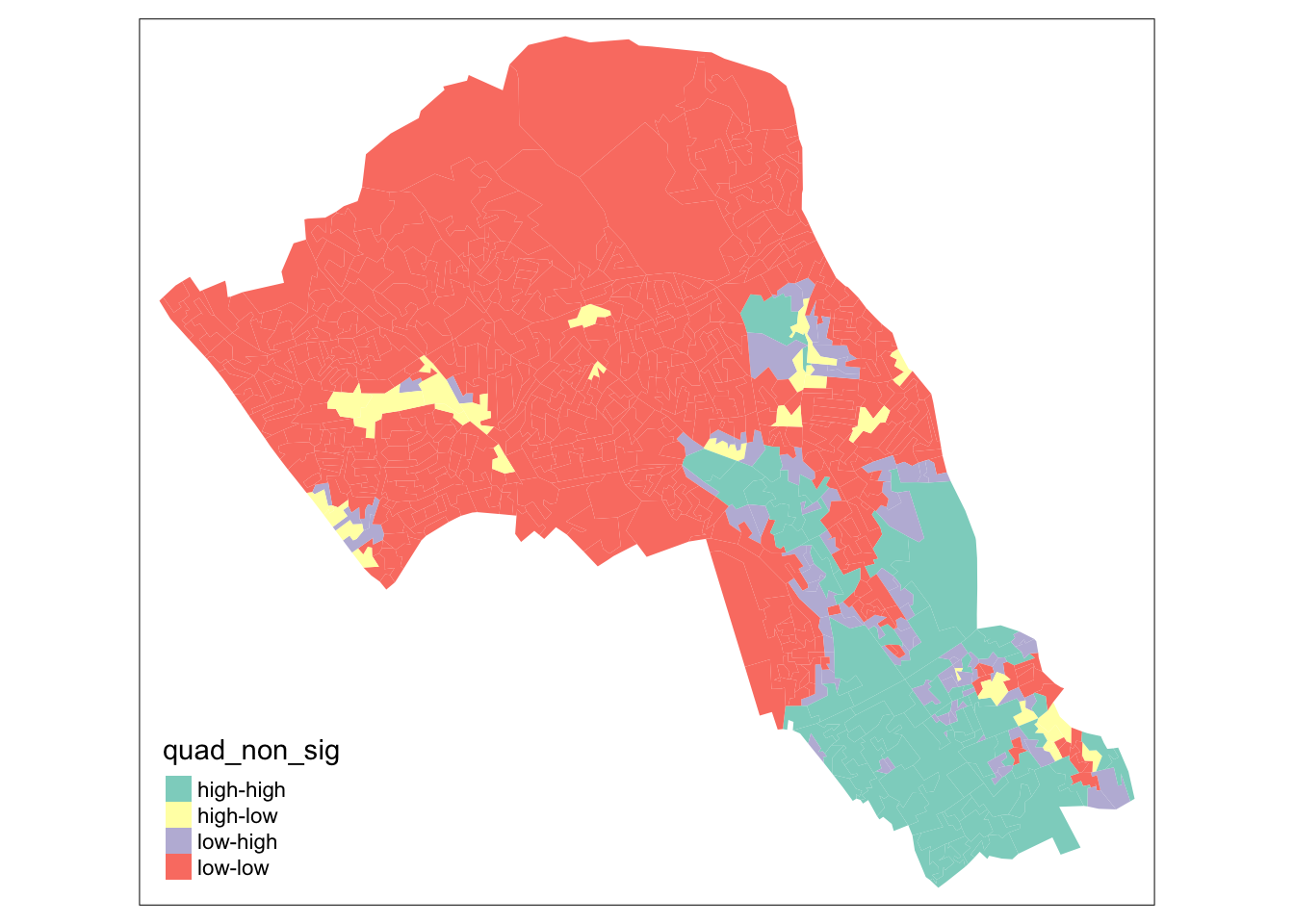
# map only the statistically significant results here
tm_shape(camden_oas_moran_stats) +
  tm_fill(col = 'quad_sig')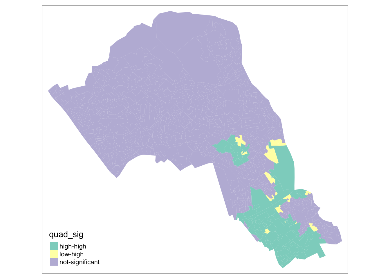
As our data are so spatially clustered we can’t see any outlier places (once we have ignored the non-significant results). This suggests that the pattern of theft from persons is not highly concentrated in very small areas or particular Output Areas, and instead is spread on a larger scale than we have used here. To go further than we have today it would be possible to run the exact same code but using a larger scale, perhaps LSOA, or Ward, and compare how this changes the Moran’s I statistics globally and locally. Or, to gain statistical significance in looking at the difference between areas getting more data perhaps over a longer timescale, where there are less areas with 0 thefts.
2.13 Tidy data
In this bonus part of this week’s session we will start by creating a tidy data set using some data from the UK 2011 Census of Population. As explained in the lecture, tidy data refers to a consistent way to structure your data in R. Tidy data, as formalised by R Wizard Hadley Wickham in his contribution to the Journal of Statistical Software is not only very much at the core of the tidyverse R package, but also of general importance when organising your data.
You can represent the same underlying data in multiple ways. The example below, taken from the the tidyverse package and described in the R for Data Science book, shows that the same data can organised in four different ways.
# load the tidyverse
library(tidyverse)
Table 1:
table1## # A tibble: 6 × 4
## country year cases population
## <chr> <int> <int> <int>
## 1 Afghanistan 1999 745 19987071
## 2 Afghanistan 2000 2666 20595360
## 3 Brazil 1999 37737 172006362
## 4 Brazil 2000 80488 174504898
## 5 China 1999 212258 1272915272
## 6 China 2000 213766 1280428583Table 2:
table2## # A tibble: 12 × 4
## country year type count
## <chr> <int> <chr> <int>
## 1 Afghanistan 1999 cases 745
## 2 Afghanistan 1999 population 19987071
## 3 Afghanistan 2000 cases 2666
## 4 Afghanistan 2000 population 20595360
## 5 Brazil 1999 cases 37737
## 6 Brazil 1999 population 172006362
## 7 Brazil 2000 cases 80488
## 8 Brazil 2000 population 174504898
## 9 China 1999 cases 212258
## 10 China 1999 population 1272915272
## 11 China 2000 cases 213766
## 12 China 2000 population 1280428583Table 3:
table3## # A tibble: 6 × 3
## country year rate
## * <chr> <int> <chr>
## 1 Afghanistan 1999 745/19987071
## 2 Afghanistan 2000 2666/20595360
## 3 Brazil 1999 37737/172006362
## 4 Brazil 2000 80488/174504898
## 5 China 1999 212258/1272915272
## 6 China 2000 213766/1280428583Table 4a:
table4a## # A tibble: 3 × 3
## country `1999` `2000`
## * <chr> <int> <int>
## 1 Afghanistan 745 2666
## 2 Brazil 37737 80488
## 3 China 212258 213766Table 4b:
table4b## # A tibble: 3 × 3
## country `1999` `2000`
## * <chr> <int> <int>
## 1 Afghanistan 19987071 20595360
## 2 Brazil 172006362 174504898
## 3 China 1272915272 1280428583None of these representations are wrong per se, however, not are equally easy to use. Only Table 1 can be considered as tidy data because it is the only table that adheres to the three rules that make a data set tidy:
- Each variable must have its own column.
- Each observation must have its own row.
- Each value must have its own cell.
.](images/week04/04_a_tidy_data.png)
Figure 2.1: A visual representation of tidy data by Hadley Wickham.
Fortunately, there are some functions in the tidyr and dplyr packages, both part of the tidyverse that will help us cleaning and preparing our data sets to create a tidy data set. The most important and useful functions are:
| Package | Function | Use to |
|---|---|---|
| dplyr | select | select columns |
| dplyr | filter | select rows |
| dplyr | mutate | transform or recode variables |
| dplyr | summarise | summarise data |
| dplyr | group by | group data into subgropus for further processing |
| tidyr | pivot_longer | convert data from wide format to long format |
| tidyr | pivot_wider | convert long format data set to wide format |
Note
Remember that when you encounter a function in a piece of R code that you have not seen before and you are wondering what it does that you can get access the documentation through ?name_of_function, e.g. ?pivot_longer. For almost any R package, the documentation contains a list of arguments that the function takes, in which format the functions expects these arguments, as well as a set of usage examples.
Now we know what constitute tidy data, we can put this into practice with an example using some data from the Office for National Statistics. Let’s say we are requested to analyse some data on the ethnic background of the UK population, for instance, because we want to get some insights into the relationship between COVID-19 and ethnic background. Our assignment is to calculate the relative proportions of each ethnic group within the administrative geography of the Middle layer Super Output Area (MSOA). In order to do this, we have access to a file that contains data on ethnicity by age group at the MSOA-level of every person in the 2011 UK Census who is 16 year or older. Download the file to your own computer and set up your data directory as usual.
Note
Make sure that after downloading you first unzip the data, for instance, using 7-Zip on Windows or using The Unarchiver on Mac OS.
File download
| File | Type | Link |
|---|---|---|
| Ethnicity by age group 2011 Census of Population | csv |
Download |
We start by making sure our tidyverse is loaded into R and using the read_csv() function to read our csv file.
# load the tidyverse
library(tidyverse)

# read data into dataframe
df <- read_csv('data/population/msoa_eth2011_ew_16plus.csv')

# inspect the dataframe: number of columns
ncol(df)
## [1] 385# inspect the dataframe: number of rows
nrow(df)## [1] 7201# inspect the dataframe: sneak peak
print(df, n_extra=2)## Warning: The `n_extra` argument of `print()` is deprecated as of pillar 1.6.2.
## Please use the `max_extra_cols` argument instead.## # A tibble: 7,201 × 385
## msoa11cd `Sex: All perso… `Sex: All perso… `Sex: All perso… `Sex: All perso…
## <chr> <dbl> <dbl> <dbl> <dbl>
## 1 E02002559 215 206 204 0
## 2 E02002560 175 170 168 1
## 3 E02002561 140 128 128 0
## 4 E02002562 160 155 154 0
## 5 E02002563 132 130 130 0
## 6 E02002564 270 263 261 0
## 7 E02002565 124 119 117 0
## 8 E02002566 150 125 117 0
## 9 E02002567 178 166 159 0
## 10 E02002568 162 159 157 0
## # … with 7,191 more rows, and 380 more variables:
## # Sex: All persons; Age: Age 16 to 17; Ethnic Group: White: Gypsy or Irish Traveller; measures: Value <dbl>,
## # Sex: All persons; Age: Age 16 to 17; Ethnic Group: White: Other White; measures: Value <dbl>,
## # …Because the data are split out over multiple columns, it is clear that the data are not directly suitable to establish the proportion of each ethnic group within the population of each MSOA. Let’s inspect the names of the columns to get a better idea of the structure of our data set.
# inspect the dataframe: column names
names(df)
## [1] "msoa11cd"
## [2] "Sex: All persons; Age: Age 16 to 17; Ethnic Group: All categories: Ethnic group; measures: Value"
## [3] "Sex: All persons; Age: Age 16 to 17; Ethnic Group: White: Total; measures: Value"
## [4] "Sex: All persons; Age: Age 16 to 17; Ethnic Group: White: English/Welsh/Scottish/Northern Irish/British; measures: Value"
## [5] "Sex: All persons; Age: Age 16 to 17; Ethnic Group: White: Irish; measures: Value"
## [6] "Sex: All persons; Age: Age 16 to 17; Ethnic Group: White: Gypsy or Irish Traveller; measures: Value"
## [7] "Sex: All persons; Age: Age 16 to 17; Ethnic Group: White: Other White; measures: Value"
## [8] "Sex: All persons; Age: Age 16 to 17; Ethnic Group: Mixed/multiple ethnic group: Total; measures: Value"
## [9] "Sex: All persons; Age: Age 16 to 17; Ethnic Group: Mixed/multiple ethnic group: White and Black Caribbean; measures: Value"
## [10] "Sex: All persons; Age: Age 16 to 17; Ethnic Group: Mixed/multiple ethnic group: White and Black African; measures: Value"
## [11] "Sex: All persons; Age: Age 16 to 17; Ethnic Group: Mixed/multiple ethnic group: White and Asian; measures: Value"
## [12] "Sex: All persons; Age: Age 16 to 17; Ethnic Group: Mixed/multiple ethnic group: Other Mixed; measures: Value"
## [13] "Sex: All persons; Age: Age 16 to 17; Ethnic Group: Asian/Asian British: Total; measures: Value"
## [14] "Sex: All persons; Age: Age 16 to 17; Ethnic Group: Asian/Asian British: Indian; measures: Value"
## [15] "Sex: All persons; Age: Age 16 to 17; Ethnic Group: Asian/Asian British: Pakistani; measures: Value"
## [16] "Sex: All persons; Age: Age 16 to 17; Ethnic Group: Asian/Asian British: Bangladeshi; measures: Value"
## [17] "Sex: All persons; Age: Age 16 to 17; Ethnic Group: Asian/Asian British: Chinese; measures: Value"
## [18] "Sex: All persons; Age: Age 16 to 17; Ethnic Group: Asian/Asian British: Other Asian; measures: Value"
## [19] "Sex: All persons; Age: Age 16 to 17; Ethnic Group: Black/African/Caribbean/Black British: Total; measures: Value"
## [20] "Sex: All persons; Age: Age 16 to 17; Ethnic Group: Black/African/Caribbean/Black British: African; measures: Value"
## [21] "Sex: All persons; Age: Age 16 to 17; Ethnic Group: Black/African/Caribbean/Black British: Caribbean; measures: Value"
## [22] "Sex: All persons; Age: Age 16 to 17; Ethnic Group: Black/African/Caribbean/Black British: Other Black; measures: Value"
## [23] "Sex: All persons; Age: Age 16 to 17; Ethnic Group: Other ethnic group: Total; measures: Value"
## [24] "Sex: All persons; Age: Age 16 to 17; Ethnic Group: Other ethnic group: Arab; measures: Value"
## [25] "Sex: All persons; Age: Age 16 to 17; Ethnic Group: Other ethnic group: Any other ethnic group; measures: Value"
## [26] "Sex: All persons; Age: Age 18 to 19; Ethnic Group: All categories: Ethnic group; measures: Value"
## [27] "Sex: All persons; Age: Age 18 to 19; Ethnic Group: White: Total; measures: Value"
## [28] "Sex: All persons; Age: Age 18 to 19; Ethnic Group: White: English/Welsh/Scottish/Northern Irish/British; measures: Value"
## [29] "Sex: All persons; Age: Age 18 to 19; Ethnic Group: White: Irish; measures: Value"
## [30] "Sex: All persons; Age: Age 18 to 19; Ethnic Group: White: Gypsy or Irish Traveller; measures: Value"
## [ reached getOption("max.print") -- omitted 355 entries ]The column names are all awfully long and it looks like the data have been split out into age groups. Further to this, the data contain within group total counts: all categories, white total, mixed/multiple ethnic group total, and so on.
Note
You can also try using View(df) or use any other form of spreadsheet software (e.g. Microsoft Excel) to browse through the data set to get a better idea of what is happening and get a better idea of the structure of the data. You first will need to understand the structure of your data set before you can start reorganising your data set.
Although the data is messy and we will need to reorganise our data set, it does look there is some form of structure present that we can exploit: the various columns with population counts for each ethnic group are repeated for each of the different age groups. This means that we can go through the data frame in steps of equal size to select the data we want: starting from column 2 (column 1 only contains the reference to the administrative geography) we want to select all 24 columns of data for that particular age group. We can create a for loop that does exactly that:
# loop through the columns of our data set
for (column in seq(2,ncol(df),24)) {

  # index number of start column of age group
  start <- column

  # index number of end column of age group
  stop <- column + 23

  # print results
  print(c(start,stop))
}
## [1] 2 25
## [1] 26 49
## [1] 50 73
## [1] 74 97
## [1] 98 121
## [1] 122 145
## [1] 146 169
## [1] 170 193
## [1] 194 217
## [1] 218 241
## [1] 242 265
## [1] 266 289
## [1] 290 313
## [1] 314 337
## [1] 338 361
## [1] 362 385For each age group in our data, the printed values should (!) correspond with the index number of the start column of the age group and the index number of the end column of the age group, respectively. Let’s do a sanity check.
# sanity check: age group 16-17 (start column)
df[,2]
## # A tibble: 7,201 × 1
## `Sex: All persons; Age: Age 16 to 17; Ethnic Group: All categories: Ethnic g…
## <dbl>
## 1 215
## 2 175
## 3 140
## 4 160
## 5 132
## 6 270
## 7 124
## 8 150
## 9 178
## 10 162
## # … with 7,191 more rows# sanity check: age group 16-17 (end column)
df[,25]## # A tibble: 7,201 × 1
## `Sex: All persons; Age: Age 16 to 17; Ethnic Group: Other ethnic group: Any …
## <dbl>
## 1 0
## 2 0
## 3 0
## 4 0
## 5 0
## 6 0
## 7 0
## 8 0
## 9 0
## 10 0
## # … with 7,191 more rows# sanity check: age group 18-19 (start column)
df[,26]## # A tibble: 7,201 × 1
## `Sex: All persons; Age: Age 18 to 19; Ethnic Group: All categories: Ethnic g…
## <dbl>
## 1 157
## 2 129
## 3 102
## 4 162
## 5 121
## 6 217
## 7 126
## 8 231
## 9 175
## 10 95
## # … with 7,191 more rows# sanity check: age group 18-19 (end column)
df[,49]## # A tibble: 7,201 × 1
## `Sex: All persons; Age: Age 18 to 19; Ethnic Group: Other ethnic group: Any …
## <dbl>
## 1 1
## 2 0
## 3 0
## 4 0
## 5 0
## 6 0
## 7 0
## 8 1
## 9 0
## 10 0
## # … with 7,191 more rowsAll seems to be correct and we have successfully identified our columns. This is great, however, we still cannot work with our data as everything is spread out over different columns. Let’s fix this by manipulating the shape of our data by turning columns into rows.
# create function
columns_to_rows <- function(df, start, stop) {

  # columns we are interested in
  col_sub <- c(1,start:stop)

  # subset the dataframe
  df_sub <- dplyr::select(df,col_sub)

  # pivot the columns in the dataframe, exclude the MSOA code column
  df_piv <- pivot_longer(df_sub,-msoa11cd)

  # rename columns
  names(df_piv) <- c('msoa11cd','age_group','count')
  return(df_piv)
}

# test
columns_to_rows(df,2,25)
## # A tibble: 172,824 × 3
## msoa11cd age_group count
## <chr> <chr> <dbl>
## 1 E02002559 Sex: All persons; Age: Age 16 to 17; Ethnic Group: All categ… 215
## 2 E02002559 Sex: All persons; Age: Age 16 to 17; Ethnic Group: White: To… 206
## 3 E02002559 Sex: All persons; Age: Age 16 to 17; Ethnic Group: White: En… 204
## 4 E02002559 Sex: All persons; Age: Age 16 to 17; Ethnic Group: White: Ir… 0
## 5 E02002559 Sex: All persons; Age: Age 16 to 17; Ethnic Group: White: Gy… 2
## 6 E02002559 Sex: All persons; Age: Age 16 to 17; Ethnic Group: White: Ot… 0
## 7 E02002559 Sex: All persons; Age: Age 16 to 17; Ethnic Group: Mixed/mul… 4
## 8 E02002559 Sex: All persons; Age: Age 16 to 17; Ethnic Group: Mixed/mul… 1
## 9 E02002559 Sex: All persons; Age: Age 16 to 17; Ethnic Group: Mixed/mul… 2
## 10 E02002559 Sex: All persons; Age: Age 16 to 17; Ethnic Group: Mixed/mul… 1
## # … with 172,814 more rowsThis looks much better. Now let’s combine our loop with our newly created function to apply this to all of our data.
# create an empty list to store our result from the loop
df_lst <- list()

# loop through the columns of our data set
for (column in seq(2,ncol(df),24)) {

  # index number of start column of age group
  start <- column

  # index number of end column of age group
  stop <- column + 23

  # call our function and assign it to the list
  df_lst[[length(df_lst)+1]] <- columns_to_rows(df,start=start,stop=stop)
}

# paste all elements from the list underneath one another
# do.call executes the function 'rbind' for all elements in our list
df_reformatted <- as_tibble(do.call(rbind,df_lst))

# and the result
df_reformatted
## # A tibble: 2,765,184 × 3
## msoa11cd age_group count
## <chr> <chr> <dbl>
## 1 E02002559 Sex: All persons; Age: Age 16 to 17; Ethnic Group: All categ… 215
## 2 E02002559 Sex: All persons; Age: Age 16 to 17; Ethnic Group: White: To… 206
## 3 E02002559 Sex: All persons; Age: Age 16 to 17; Ethnic Group: White: En… 204
## 4 E02002559 Sex: All persons; Age: Age 16 to 17; Ethnic Group: White: Ir… 0
## 5 E02002559 Sex: All persons; Age: Age 16 to 17; Ethnic Group: White: Gy… 2
## 6 E02002559 Sex: All persons; Age: Age 16 to 17; Ethnic Group: White: Ot… 0
## 7 E02002559 Sex: All persons; Age: Age 16 to 17; Ethnic Group: Mixed/mul… 4
## 8 E02002559 Sex: All persons; Age: Age 16 to 17; Ethnic Group: Mixed/mul… 1
## 9 E02002559 Sex: All persons; Age: Age 16 to 17; Ethnic Group: Mixed/mul… 2
## 10 E02002559 Sex: All persons; Age: Age 16 to 17; Ethnic Group: Mixed/mul… 1
## # … with 2,765,174 more rowsNow the data is in a much more manageable format, we can move on with preparing the data further. We will start by filtering out the columns (now rows!) that contain all categories and the within group totals. We will do this by cleverly filtering our data set on only a part of the text string that is contained in the age_group column of our dataframe using a regular expression. We further truncate the information that is contained in the age_group column to make all a little more readable.
# filter rows
# this can be a little slow because of the regular expression!
df_reformatted <- filter(df_reformatted,!grepl('*All categories*',age_group))
df_reformatted <- filter(df_reformatted,!grepl('*Total*',age_group))

# create variable that flags the 85 and over category
# this can be a little slow because of the regular expression!
df_reformatted$g <- ifelse(grepl('85',as.character(df_reformatted$age_group)),1,0)

# select information from character 41 (85 and over category) or from character 38
df_reformatted <- mutate(df_reformatted,group = ifelse(g==0,substr(as.character(age_group),38,500),
                                                            substr(as.character(age_group),41,500)))

# remove unnecessary columns
df_reformatted <- dplyr::select(df_reformatted, -age_group, -g)
We are now really getting somewhere, although in order for our data to be tidy each variable must have its own column. We also want, within each ethnic group, to aggregate the individual values within each age group.
# pivot table and aggregate values
df_clean <- pivot_wider(df_reformatted,names_from=group,values_from=count,values_fn=sum)

# rename columns
# names are assigned based on index values, so make sure that the current column names match the
# order of the new colum names otherwise our whole analysis will be wrong!
names(df_clean) <- c('msoa11cd','white_british','white_irish','white_traveller','white_other','mixed_white_black_caribbean',
                     'mixed_white_black_african','mixed_white_asian','mixed_other','asian_indian','asian_pakistani',
                     'asian_bangladeshi','asian_chinese','asian_other','black_african','black_caribbean','black_other',
                     'other_arab','other_other')

# tidy data
df_clean
## # A tibble: 7,201 × 19
## msoa11cd white_british white_irish white_traveller white_other
## <chr> <dbl> <dbl> <dbl> <dbl>
## 1 E02002559 6775 17 27 51
## 2 E02002560 4688 11 8 31
## 3 E02002561 4609 20 3 55
## 4 E02002562 4653 4 6 131
## 5 E02002563 4369 13 2 38
## 6 E02002564 7320 11 3 73
## 7 E02002565 4274 16 2 96
## 8 E02002566 4713 33 24 308
## 9 E02002567 5344 17 42 111
## 10 E02002568 4583 29 6 100
## # … with 7,191 more rows, and 14 more variables:
## # mixed_white_black_caribbean <dbl>, mixed_white_black_african <dbl>,
## # mixed_white_asian <dbl>, mixed_other <dbl>, asian_indian <dbl>,
## # asian_pakistani <dbl>, asian_bangladeshi <dbl>, asian_chinese <dbl>,
## # asian_other <dbl>, black_african <dbl>, black_caribbean <dbl>,
## # black_other <dbl>, other_arab <dbl>, other_other <dbl>Finally. We now have a tidy data set that we can work with!
2.14 Assignment
Part A
Since we went through all the trouble of cleaning and creating this file, now try and use the cleaned data set to create a table that, for each MSOA, contains the proportions of the population belonging to each of the ethnic groups in the UK 2011 Census of Population. It could look something like this:
| msoa11cd | white_british | white_irish | etc. |
|---|---|---|---|
| E02002562 | 0.74 | 0.03 | … |
| E02002560 | 0.32 | 0.32 | … |
Tips
- First think what you what steps you would need to take in order to get the group proportions. Write them down on a piece of paper if you like. Once you have identified the steps, then start coding.
- Conduct sanity checks. Every time you have written a line of code, check the results to see if the code did indeed give the result that you expected to get.
- Google is your friend. Do not be afraid to search for specific solutions and suggestions, chances are that there have been other people who have faces similar problems and posted their questions on stackoverflow.
Part B
Further to calculating the proportions of the population belonging to each of the ethnic groups in the UK 2011 Census of Population, we also want to make a choropleth map at district level of the UK population that is older than 60 (as a proportion of the total population within each district). For this analysis we have available one data set with the administrative boundaries of the UK 2020 Local Authority Districts administrative geography and we have a csv file that holds population estimates for the UK in 2019. Use everything you have learned over the past weeks to produces this map. Some tips:
Tips
- Inspect both the shapefile and the
csvfile to get an idea of how your data look like. Use any tool you like to do this inspection (ArcGIS, R, QGIS, Microsoft Excel, etc.). - The
csvfile does contain a mix of administrative geographies, and you will need to do some data cleaning by filtering out Country, County, Metropolitan County, and Region before you link the data to the shapefile. - You are in charge of deciding what software you want to use to visualise the data (ArcGIS, R, QGIS, etc.).
- You now have to make your own decisions on how to go about this problem. Although this practical has so far covered some of the functions and strategies you might need, the data cleaning and data preparation process is not the same.
2.15 Attributions
This week’s content and practical uses content and inspiration from:
- Long, Alfie. 2020. Spatial autocorrelation. https://github.com/jtvandijk/GEOG0114_20202021/blob/master/04-week04.Rmd
- Gimond, Manuel. 2021. Spatial autocorrelation in R. https://mgimond.github.io/Spatial/spatial-autocorrelation-in-r.html