Getting started

R is a programming language originally designed for conducting statistical analysis and creating graphics. The major advantage of using R is that it can be used on any computer operating system, and is free for anyone to use and contribute to. Because of this, it has rapidly become the statistical language of choice for many academics and has a large user community with people constantly contributing new packages to carry out all manner of statistical, graphical, and geographical tasks. In this tutorial, we will guide you through installing R on your computer and review the basics of interacting with the language and its functions.

Installation of R

Installing R takes a few relatively simple steps involving two pieces of software. First there is the R programming language itself. Follow these steps to get it installed on your computer:

1. Navigate in your browser to the download page: [Link]
2. If you use a Windows computer, click on Download R for Windows. Then click on base. Download and install R 4.4.x for Windows. If you use a Mac computer, click on Download R for macOS and download and install R-4.4.x.arm64.pkg for Apple silicon Macs or R-4.4.x.x86_64.pkg for older Intel-based Macs.

That is it! You now have successfully installed R onto your computer. To make working with the R language a little bit easier we also need to install something called an Integrated Development Environment (IDE). We will use RStudio Desktop:

1. Navigate to the official webpage of RStudio: [Link]
2. Download and install RStudio on your computer.

In case you do not have access to a laptop or encounter issues with the installation process, RStudio is also available through Desktop@UCL Anywhere as well as that it can be accessed on UCL computers across campus.

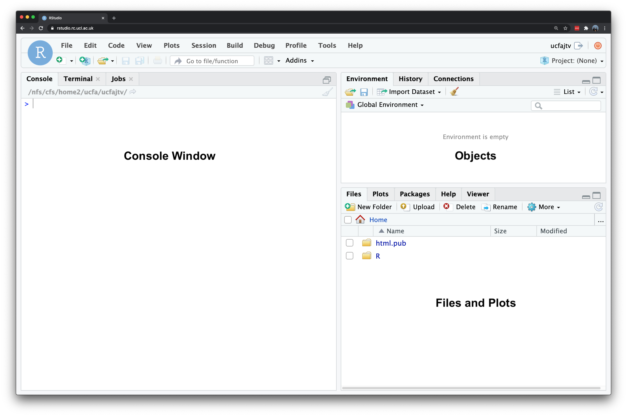
After this, start RStudio to see if the installation was successful. Your screen should look something like what is shown in Figure 1.

Figure 1: The RStudio interface.

The main panes that we will be using are:

Window	Purpose
Console	Where we write one-off code such as installing packages.
Files	Where we can see where our files are stored on our computer system.
Environment	Where our variables or objects are kept in memory.
Plots	Where the outputs of our graphs, charts and maps are shown.

Customisation of R

Now we have installed R and RStudio, we need to customise R. Many useful R functions come in packages, these are free libraries of code written and made available by other R users. This includes packages specifically developed for data cleaning, data wrangling, visualisation, mapping, and spatial analysis. To save us some time later on, we will install the R packages that we will need during the module in one go.

Start RStudio, and copy and paste the following code into the console window. You can execute the code by pressing the Return button on your keyboard. Depending on your computer’s specifications and the internet connection, this may take a short while.

R code

# install packages
install.packages(c('tidyverse', 'janitor', 'descr', 'ggcorrplot','patchwork','easystats'))

R libraries installed through CRAN are typically pre-compiled, meaning that these packages can be easily installed on your machine without additional steps. However, when attempting to install an R library that requires compilation, additional software must be installed. For Windows users, RTools provides the necessary tools for building R packages from source. MacOS users should install Xcode as well as the GNU Fortran compiler.

Once you have installed the packages, we need to check whether we can in fact load them into R. Copy and paste the following code into the console, and execute by pressing Return on your keyboard.

R code

# load packages
library(tidyverse)
library(janitor)
library(descr)
library(ggcorrplot)
library(patchwork)
library(easystats)

You will see some information printed to your console but as long as you do not get any of the messages below, the installation was successful. If you do get any of the messages below it means that the package was not properly installed, so try to install the package in question again.

• Error: package or namespace load failed for <packagename>
• Error: package '<packagename>' could not be loaded
• Error in library(<packagename>) : there is no package called '<packagename>'

Many packages require additional software components, known as dependencies, to function properly. Occasionally, when you install a package, some of these dependencies are not installed automatically. When you then try to load a package, you might encounter error messages that relate to a package that you did not explicitly loaded or installed. If this is the case, it is likely due to a missing dependency. To resolve this, identify the missing dependency and install it using the command install.packages('<dependencyname>'). Afterwards, try loading your packages again.

Getting started with R

Unlike traditional statistical analysis software like Microsoft Excel or IBM SPSS Statistics, which often rely on point-and-click interfaces, R requires users to input commands to perform tasks such as loading datasets and fitting models. This command-based approach is typically done by writing scripts, which not only document your workflow but also allow for easy repetition of tasks.

Let us begin by exploring some of R’s built-in functionality through a simple exercise: creating a few variables and performing basic mathematical operations.

In your RStudio console, you will notice a prompt sign > on the left-hand side. This is where you can directly interact with R. If any text appears in red, it indicates an error or warning. When you see the >, it means R is ready for your next command. However, if you see a +, it means you have not completed the previous line of code. This typically happens when brackets are left open or a command is not properly finished in the way R expected.

At its core, every programming language can be used as a powerful calculator. Type in 10 * 12 into the console and execute.

R code

# multiplication
10 * 12

[1] 120

Once you press return, you should see the answer of 120 returned below.

Storing variables

Instead of using raw numbers or standalone values, it is more effective to store these values in variables, which allows for easy reference later. In R, this process is known as creating an object, and the object is stored as a variable. To assign a value to a variable, use the <- syntax. Let us create two variables to experiment with this

Type in ten <- 10 into the console and execute.

R code

# store a variable
ten <- 10

You will see nothing is returned to the console. However, if you check your environment window, you will see that a new variable has appeared, containing the value you assigned.

Type in twelve <- 12 into the console and execute.

R code

# store a variable
twelve <- 12

Again, nothing will be returned to the console, but be sure to check your environment window for the newly created variable. We have now stored two numbers in our environment and assigned them variable names for easy reference. R stores these objects as variables in your computer’s RAM memory, allowing for quick processing. Keep in mind that without saving your environment, these variables will be lost when you close R and you would need to run your code again.

Now that we have our variables, let us proceed with a simple multiplication. Type in ten * twelve into the console and execute.

R code

# using variables
ten * twelve

[1] 120

You should see the output in the console of 120. While this calculation may seem trivial, it demonstrates a powerful concept: these variables can be treated just like the values they contain.

Next, type in ten * twelve * 8 into the console and execute.

R code

# using variables and values
ten * twelve * 8

[1] 960

You should get an answer of 960. As you can see, we can mix variables with raw values without any problems. We can also store the output of variable calculations as a new variable.

Type output <- ten * twelve * 8 into the console and execute.

R code

# store output 
output <- ten * twelve * 8

Because we are storing the output of our calculation to a new variable, the answer is not returned to the screen but is kept in memory.

Accessing variables

We can ask R to return the value of the output variable by simply typing its name into the console. You should see that it returns the same value as the earlier calculation.

R code

# return value 
output

[1] 960

Text variables

We can also store variables of different data types, not just numbers but text as well.

Type in str_variable <- "Hello GEOG0018" into the console and execute.

R code

# store a variable
str_variable <- 'Hello GEOG0018'

We have just stored our sentence made from a combination of characters. A variable that stores text is known as a string or character variable. These variables are always denoted by the use of single ('') or double ("") quotation marks.

Type in str_variable into the console and execute.

R code

# return variable
str_variable

[1] "Hello GEOG0018"

You should see our entire sentence returned, enclosed in quotation marks ("").

Calling functions

We can call functions on our variable. For example, we can ask R to print our variable, which will give us the same output as accessing it directly via the console.

Type in print(str_variable) into the console and execute.

R code

# printing a variable
print(str_variable)

[1] "Hello GEOG0018"

You can type ?print into the console to learn more about the print() function. This method works with any function, giving you access to its documentation. Understanding this documentation is crucial for using the function correctly and interpreting its output.

R code

# open documentation of the print function
?print

In many cases, a function will take more than one argument or parameter, so it is important to know what you need to provide the function with in order for it to work. For now, we are using functions that only need one required argument although most functions will also have several optional or default parameters.

Inspecting variables

Within the base R language, there are various functions that have been written to help us examine and find out information about our variables. For example, we can use the typeof() function to check what data type our variable is.

Type in typeof(str_variable) into the console and execute.

R code

# call the typeof() function
typeof(str_variable)

[1] "character"

You should see the answer: character. As evident, our str_variable is a character data type. We can try testing this out on one of our earlier variables too.

Type in typeof(ten) into the console and execute.

R code

# call the typeof() function 
typeof(ten)

[1] "double"

You should see the answer: double. Alternatively, we can check the class of a variable by using the class() function.

Type in class(str_variable) into the console and execute.

R code

# call the class() function 
class(str_variable)

[1] "character"

In this case, you will see the same result as before because, in R, both the class and type of a string are character. Other programming languages might use the term string instead, but it essentially means the same thing.

Type in class(ten) into the console and execute.

R code

# call the class() function 
class(ten)

[1] "numeric"

In this case, you will get a different result because the class of this variable is numeric. Numeric objects in R can be either doubles (decimals) or integers (whole numbers). You can test whether the ten variable is an integer by using specific functions designed for this purpose.

Type in is.integer(ten) into the console and execute.

R code

# call the integer() function
is.integer(ten)

[1] FALSE

You should see the result FALSE. As we know from the typeof() function, the ten variable is stored as a double, so it cannot be an integer.

Whilst knowing how to distinguish between different data types might not seem important now, the difference betwee a double and an integer can quite easily lead to unexpected errors.

We can also check the length of our a variable.

Type in length(str_variable) into the console and execute.

R code

# call the length() function 
length(str_variable)

[1] 1

You should get the answer 1 because we only have one set of characters. We can also determine the length of each set of characters, which tells us the length of the string contained in the variable.

Type in nchar(str_variable) into the console and execute.

R code

# call the nchar() function
nchar(str_variable)

[1] 14

You should get an answer of 14.

Creating multi-value objects

Variables are not constricted to one value, but can be combined to create larger objects. Type in two_str_variable <- c("This is our second variable", "It has two parts to it") into the console and execute.

R code

# store a new variable 
two_str_variable <- c("This is our second string variable", "It has two parts to it")

In this code, we have created a new variable using the c() function, which combines values into a vector or list. We provided the c() function with two sets of strings, separated by a comma and enclosed within the function’s parentheses.

Let us now try both our length() and nchar() on our new variable and see what the results are:

R code

# call the length() function 
length(two_str_variable)

[1] 2

# call the nchar() function
nchar(two_str_variable)

[1] 34 22

You should notice that the length() function now returned a 2 and the nchar() function returned two values: 34 and 22.

You may have noticed that each line of code in the examples includes a comment explaining its purpose. In R, comments are created using the hash symbol #. This symbol instructs R to ignore the commented line when executing the code. Comments are useful for understanding your code when you revisit it later or when sharing it with others.

Extending the concept of multi-value objects to two dimensions results in a dataframe. A dataframe is the de facto data structure for most tabular data. We will use functions from the tidyverse library, a suite of packages to load tabular data and conduct data analysis.

Within the tidyverse, dataframes are referred to as tibbles. Some of the most important and useful functions come from the tidyr and dplyr packages, including:

Package	Function	Use to
dplyr	select()	select columns
dplyr	filter()	select rows
dplyr	mutate()	create, transform, or recode variables
dplyr	summarise()	summarise data
dplyr	group_by()	group data into subgroups for further processing
tidyr	pivot_longer()	convert data from wide format to long format
tidyr	pivot_wider()	convert long format dataset to wide format

For more information on the tidyverse you can refer to www.tidyverse.org.

We will be using these functions in the coming weeks, so ensure you are familiar with what they do and how they work.

Before you leave

This introductory tutorial did not cover anything new that you have not encountered in last year’s modules. However, since it has been some time, you should now have R and RStudio installed (again?) and working on your computer, or at the very least, be able to access RStudio via Desktop@UCL Anywhere with the necessary libraries installed. Now that you are up to speed, time for some real action by using R for some data analysis